Artificial Neural Networks and its Application to Industrial Fault Diagnosis of Connecting Rods in Compressors: Introduction and Applications

Creating neural networks by using MATLAB and applying it to solve technical problems like pattern recognition for correct sorting of parcels and classification for fault diagnosis of compressor connecting rods.

Neuron Model and Transfer Functions

1. Neuron Model

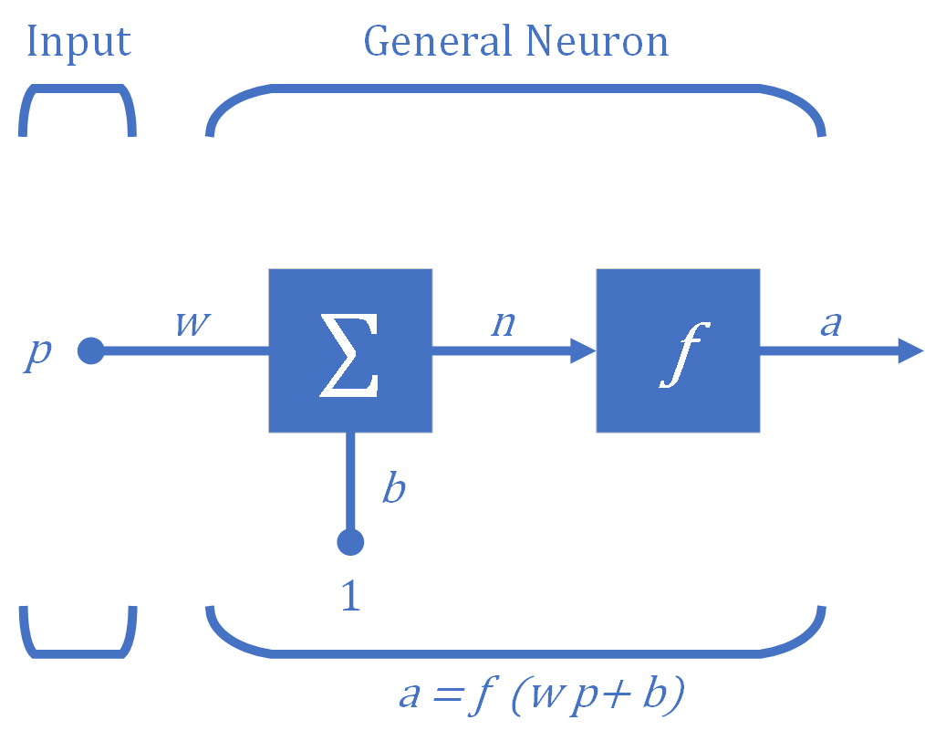
The fundamental building block for neural networks is the single-input neuron illustrated in Figure 1. There are three functional operations in a neuron.

• First, the scalar input $p$ is multiplied by the scalar weight $w$ to form the scalar product $wp$. This process is called the weight function.
• Second, the weighted input $wp$ is added to the scalar bias $b$ (also called "offset"), which is like a weight but with a constant input of $1$, to form the net input $n$. This process is called the net input function.
• Finally, the net input $n$ is passed through the transfer function $f$ (also called "activation function"), which produces the scalar output $a$. This process is called the transfer function. Without specifying the transfer function the output of the neuron cannot be determined.

2. Transfer Functions

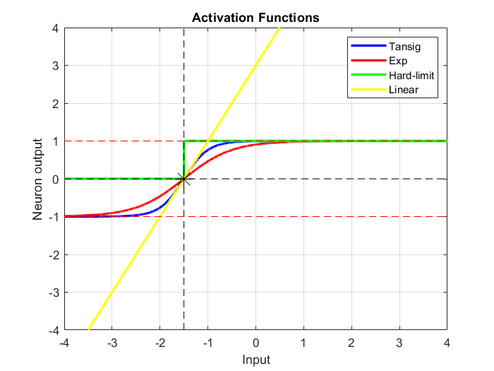
There are numerous commonly used activation functions. In the following code four activation functions are computed and plotted for a net input $n$:

1. Hyperbolic tangent sigmoid transfer function: $$a=f\left(n\right)=\mathrm{tansig}\left(n\right)=\frac{2}{1+e^{-2n} }-1$$
2. Exponential transfer function: $$a=f\left(n\right)=\frac{2}{1+e^{-n} }-1$$
3. Hard-limit transfer function: $$a=f\left(n\right)=\mathrm{hardlim}\left(n\right)=\left\lbrace \begin{array}{ll} 1 & \mathrm{if}\;n\ge 0\\ 0 & \mathrm{otherwise} \end{array}\right.$$
4. Linear transfer function: $$a=f\left(n\right)=\mathrm{purelin}\left(n\right)=n$$

where the net input $n=\mathbf{Wp}+b=2p+3$ when the weight $w$ on the single input $p$ is $2$ and the bias $b$ is $3$.

The exponential transfer function is normalized and offset from zero so that the output ranges from $−1$ to $1$.

The hyperbolic tangent sigmoid transfer function (tansig or tanh) and the exponential transfer function are very similar. They put bounds on the output. In this case, within the range $−3 ≤ n < 1$, where they return the function of the input. Outside those bounds, they return $-1$ or $1$.

The hard-limit transfer function (hardlim) returns $0$ if the value is less than a threshold value and $1$ if it is greater than or equal to that threshold, here $−1.5$.

The linear transfer function simply calculates the neuron’s output by simply returning the value $n$ passed to it.

The following code computes and plots these four activation functions for a net input $n$:

The central idea of neural networks is adjusting the adjustable scalar parameters, $w$ and $b$, of the neuron so that the network exhibits some desired or interesting behavior. This procedure is referred to as perceptron learning rule or training algorithm.

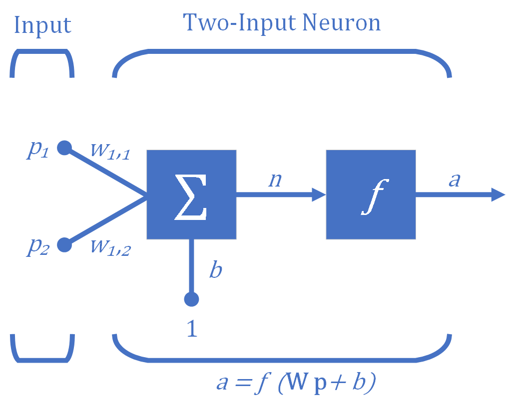
Multiple-Input Neuron

The simple neuron can be extended to handle inputs that are vectors. A neuron with a single Two-element input vector $(R=2)$ is shown in Figure 3, where the individual input elements $p_1$ and $p_2$ are multiplied by weights $w_{1,1}$ and $w_{1,2}$ of the neuron (here, there is one neuron) and the weighted values are fed to the summing junction. Their sum is simply $\textbf{Wp}$, the dot product, which is simply the sum of the componentwise products of the vector components, of the (single row) matrix $\textbf{W}$ and the vector $\textbf{p}$. The neuron has a bias (offset) $b$, which is summed with the weighted inputs to form the net input $n$. The net input $n$ is the argument of the transfer function $f$.

A decision boundary is determined by the input vectors for which the net input $n$ is zero.

This defines a boundary in the input space (feature space), a linear separator, dividing the input space into two parts. An input space comprises all potential sets of values for input. If the inner product of the weight matrix $\textbf{W}$ (a single row vector in this case) with the input vector $\textbf{p}$ is greater than or equal to $-b$, the output will be positive $(n>1)$, otherwise the output will be negative $(n<1)$. Figure 4 illustrates this for the case where $b = -3$. The blue line in the figure, the linear separator,in three dimensions, it is called a plane or hyperplane, and it represents all points for which the net input $n$ is equal to zero and thus, in the input-output space, the outcome of transfer function $f$, in this case, the hyperbolic tangent sigmoid transfer function, is also zero. The shaded region contains all input vectors for which the output of the network will be closer or equal to $1$. The output will be closer or equal to $-1$ for all other input vectors (the unshaded region).

Basically, there are an infinite set of equations all of which represent the same separator, because multiplying both sides of the equation by any number won’t affect the equality.

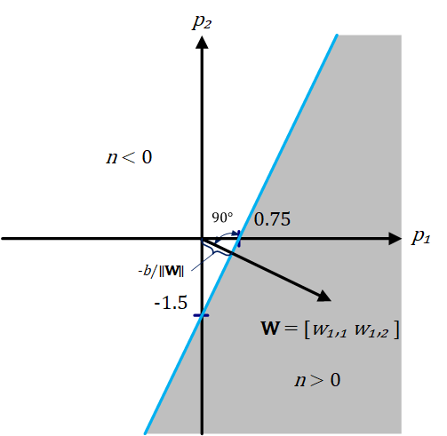
The decision boundary, a hyperplane, will always be orthogonal to the weight matrix, and the position of the boundary can be shifted by changing $b$. To clarify, from the definition of orthogonality in mathematics, two vectors are orthogonal in Euclidean space if and only if their dot product is zero, i.e. they make an angle of $90°$. Also, from the definition of hyperplane in geometry, a hyperplane is a subspace whose dimension is one less than that of its ambient space (surrounding space). So in a two dimensional space a hyperplane would be a line.

Considering an $n$-dimensional space, a plane is defined by the equation:

where $\textbf{w}$ and $\textbf{p}$ are both length-$n$ vectors. $\textbf{w}$ is a vector orthogonal to the plane which contains the vector $\textbf{p}$ and $b$ is proportional to the perpendicular distance from the origin to the plane (the decision boundary). The constant of proportionality is the negative of the magnitude of the normal vector.

To summarize, in general, the goal of learning in a single output perceptron is to adjust the separating hyperplane (i.e., linear decision boundary) that divides an $n$-dimensional “input space,” where $n$ is the number of net inputs, by modifying the weights and the bias until all the input vectors with target value $1$ are on one side of the hyperplane, and all the input vectors with target value $0$ or $-1$, depending on the activation function, are on the other side of the hyperplane. In a nework with multiple neurons, $\textbf{W}$ is a matrix consisting of a number of row vectors, each of which will be used in an equation similar to the above one. There will be one boundary for each row of $\textbf{W}$.

The key property of the single-neuron perceptron, therefore, is that it can separate input vectors into two categories. Because the boundary is linear, the single-layer perceptron can only be used to classify inputs that are linearly separable (can be separated by a linear boundary).

To define a network the following problem specifications are helpful:

1. Number of network inputs = number of problem inputs
2. Number of neurons in output layer = number of problem outputs
3. Output layer transfer function choice at least partly determined by problem specification of the outputs

Problem Description

Calculating the output of a simple neuron.

Steps

1. Defining neuron parameters
2. Defining the input vector
3. Calculating neuron output
4. Plotting neuron output over the range of inputs

1. Defining neuron parameters

Considering a two-input perceptron with one neuron as shown in Figure 2 above and assigning the following values for the weights and bias as follows:

In the case of single neuron, the scalar net input $n$ to the tranfer function $f$, which produces the scalar neuron output $a$, is given by:

• $$ n=\ \mathit{\mathbf{p}}*\ {\mathit{\mathbf{W}}}^T +b $$
• $$ ={\left[\begin{array}{cc} p_1 & p_2 \end{array}\right]}\cdot {\left[\begin{array}{cc} 4 & -2 \end{array}\right]^{T}} -3 $$
• $$ =4p_1 -2p_2 -3 $$

2. Defining the input vector

3. Calculating neuron output

The output of this network is determined by a transfer function, for example the hyperbolic tangent sigmoid transfer function tansig.

4. Plotting neuron output over the range of inputs

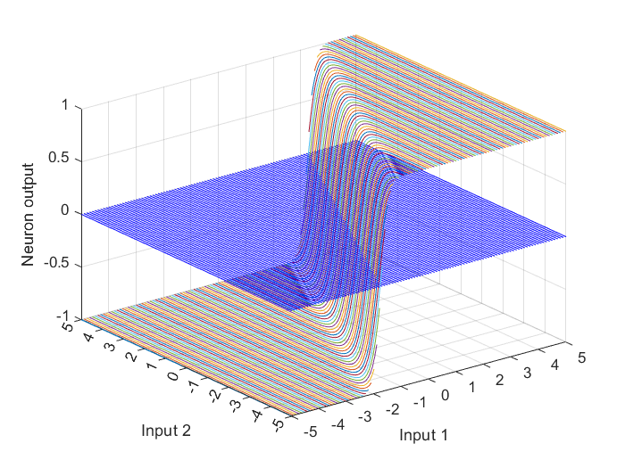
The above described neuron with a vector input could be illustrated in the input-output space by graphing the network output over range of input values for $p_1$ and $p_2$, as shown in Figure 5. For this purpose, the MATLAB function meshgrid is used here to create two matrices $p_1$ and $p_2$, each with a size of $101\times101$. The function meshgrid returns 2-D grid coordinates based on the coordinates contained in the assigned vector between the parentheses. $p_1$ is a matrix where each row is a copy of the assigned vector, and $p_2$ is a matrix where each column is a copy of the assigned vector.

To find the neuron output, the function is evaluated at the input values resulting, in this case, from the equation $4p_1 -2p_2 -3$.

The types of the inputs and outputs depend on the function, in this case: the hyperbolic tangent sigmoid transfer function tansig, which takes a matrix of net input column vector and returns a column vector matrix of the same size consisting of the elements of the input column vector where each element of it is squashed from the interval $[-inf \quad inf]$ to the interval $[-1 \quad 1]$ with an “S-shaped” curve.

To plot the inputs and outputs in a 3-D plot by using MATLAB function plot3, the inputs and the output matrices must have at least one dimension that is same size. However, here the input and output matrices don’t have a same size dimension, thus, reshape function is used to reshape the output column vector a and return a reshaped array a of the size: $length\left(p_{1} \right) \times length\left(p_{2} \right)$.

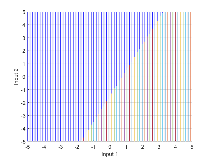
The next lines of code shows the top view of the input-output space plot, Figure 6, which is the input-space, where the intersection of the decision boundary with the transfer function curves is a line, similar to the linear separator previously illustrated in Figure 4.

Multiple-Neuron Perceptron

As mentioned earlier, each neuron has a single decision boundary. A single-neuron perceptron can classify input vectors into two categories, as its output can be either $0$ or $1$. A multiple-neuron perceptron can classify inputs into many categories. Each category is represented by a different output vector. Since each element of the output vector can be either $0$ or $1$, there are a total of possible $2^S$ categories, where $S$ is the number of neurons. For a perceptron with multiple neurons the decision boundary for each neuron $i$ will be defined by:

Perceptron Learning Rule

By learning rule is meant a procedure (an algorithm) for modifying the weights and biases of a network. (This procedure is also referred to as a training algorithm). The purpose of the learning rule is to train the network to perform some task, like solving a classification problem. There are many types of neural network training algorithms (learning rules). They fall into three broad categories: supervised learning, unsupervised learning and reinforcement (or graded) learning.

In supervised learning, the learning rule is provided with a set of examples (the training set) of proper network behavior (inputs and their target outputs):

where $\textbf{p}_q$ is an input to the network and $\textbf{t}_q$ is the corresponding correct (target) output. As the inputs are applied to the network, the network outputs are compared to the targets. The learning rule is then used to adjust the weights and biases of the network in order to move the network outputs closer to the targets.

Reinforcement learning is similar to supervised learning, except that, instead of being provided with the correct output for each network input, the algorithm is only given a grade. The grade (or score) is a measure of the network performance over some sequence of inputs.

In unsupervised learning, the weights and biases are modified in response to network inputs only. There are no target outputs available.

To begin the training and to construct the learning rules, some initial values are assigned for the network parameters (weights and biases). Then, the input vectors are presented to the network one by one. Each time the network doesn’t return the correct value (the target output associated with the input), the weight vector is altered so that it points more toward the input vector. If the network returns the correct value, then there is no need to alter anything. In this way, a single expression is found that resembles a unified learning rule. For this, firs a new variable is defined, the perceptron error $e$:

where $e$ is the wrong output value (also called error). It equals to $0$ when the network returns the correct output $(t=a)$. In this way, the unified learning rule for multiple-neuron perceptrons in matrix notation is:

and

Although the perceptron learning rule is simple, it is quite powerful. It will always converge to weights that accomplish the desired classification (assuming that such weights exist).

An Illustrative Example

The following example is to show how the architectures described in the previous sections can be used to solve a simple practical problem,- a pattern recognition problem, by using three different neural network architectures; a single-layer perceptron (feedforward network) with a symmetric hard-limit transfer function hardlims, a Hamming network (competitive network) and a Hopfield network (recurrent associative memory network).

Problem Description

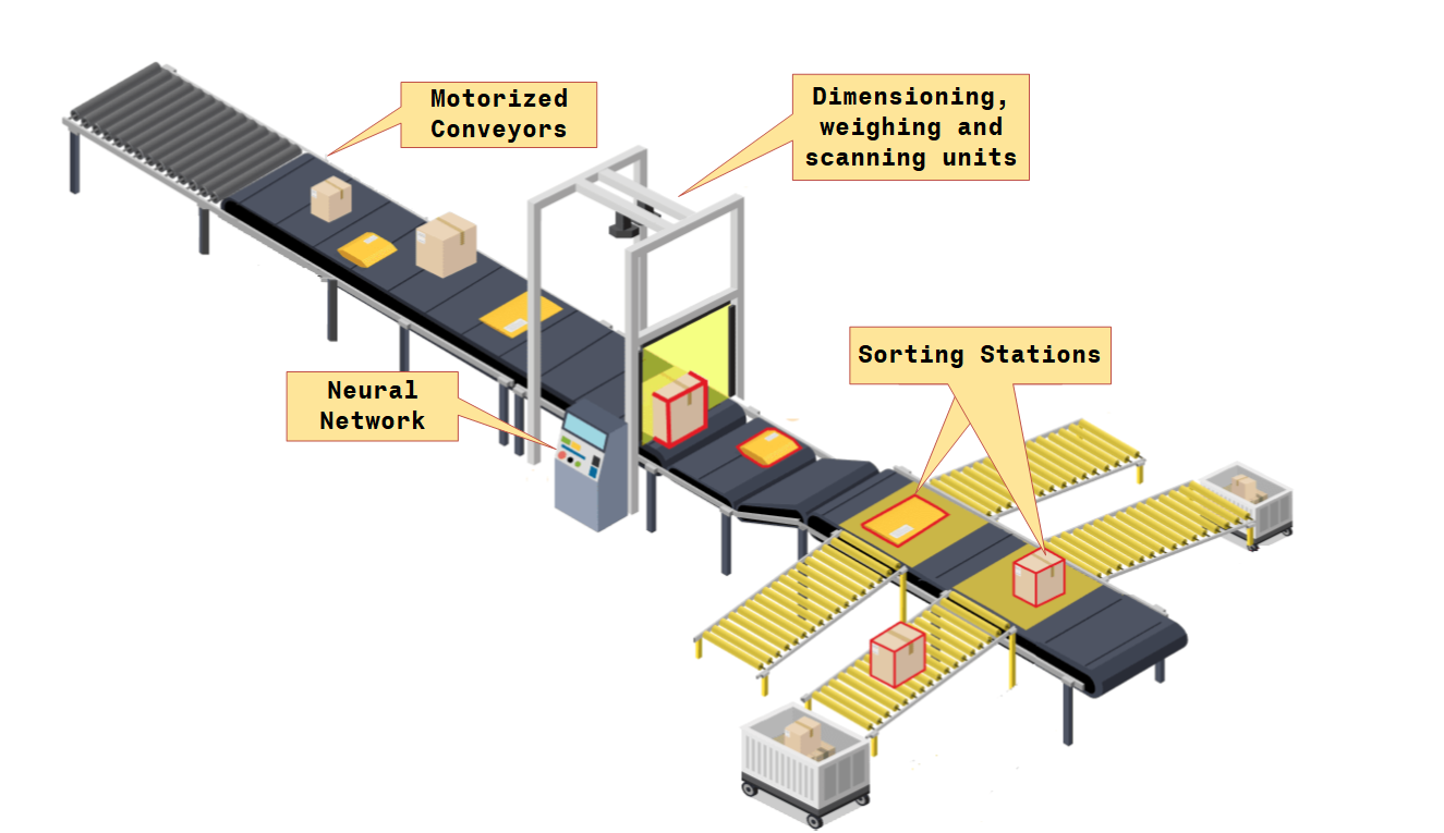
A central processing station has a parcel sorting machine that through scanning, volumetric and weighing technologies can identify and accurately profile parcels, as shown in Figure 7. When parcels reach a central processing station, various types of parcels may be mixed together. The goal is to sort the parcels according to type. There is a conveyer belt on which the parcel is loaded. This conveyer passes through a set of sensors, that measure three properties of the parcel: size, shape and weight. Considering that these sensors will output two values $1$ and $-1$. The size sensor will output a $1$ if the parcel is a medium size parcel and a $-1$ if it is a packet. The shape sensor will output a $1$ if the parcel is approximately round and a $-1$ if it is more rectangular. The weight sensor will output a $1$ if the parcel is more than $10$ kilograms and a $-1$ if the parcel is equal to or less than $10$ kilograms.

The three sensor outputs will then be input to a neural network. The purpose of the network is to decide which kind of parcel is on the conveyor, so that the parcel can be directed to the correct direction. To make the problem even simpler, it is assumed that there are only two types of parcels on the conveyor: Type A (medium size, rectangular, heavier than 10 kilograms) and Type B (packet, rectangular, equal or less than 10 kilograms).

Objectives

1. Designing a perceptron (feedforward network) to recognize patterns
2. Finding and sketching a decision boundary for the perceptron network that will recognize these prototype patterns
3. Finding weights and bias which will produce this decision boundary
4. Designing a Hamming network (competitive network) to recognize these patterns
5. Designing a Hopfield network (recurrent associative memory network) to recognize these patterns

Solution

1. Designing a perceptron (feedforward network) to recognize patterns

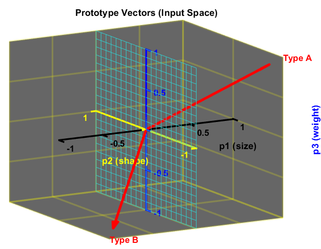
As each parcel passes through the sensors it can be represented by a three-dimensional vector. The first element of the vector will represent size, the second element will represent shape and the third element will represent weight:

Therefore, a Type A prototype would be represented by the vector

and a Type B prototype would be represented by the vector

The neural network will receive one three-dimensional input vector for each parcel on the conveyer and must make a decision as to whether the parcel is of Type A $(\textbf{p}_1)$ or Type B $(\textbf{p}_2)$.

Because there are only two categories, we can use a single-neuron perceptron. The vector inputs are three-dimensional $(R=3)$, therefore the perceptron equation will be

2. Finding and sketching a decision boundary

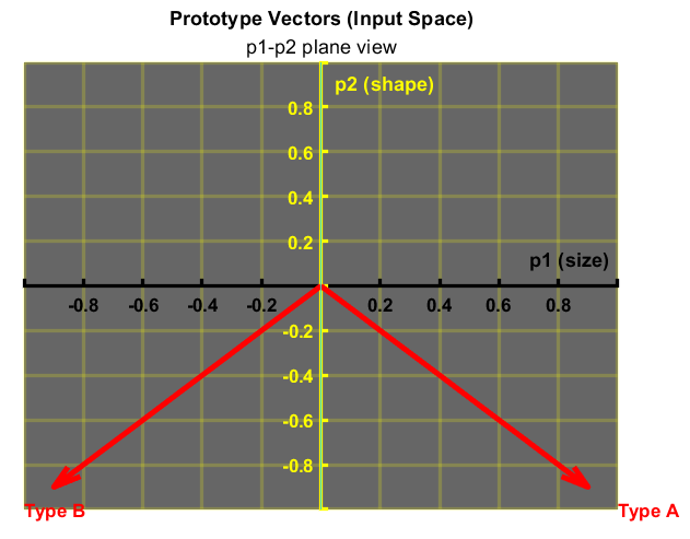
The bias and the elements of the weight matrix are chosen so that the perceptron will be able to distinguish between parcels of Type A and of Type B. For example, the perceptron is configured so that the output will be $1$ when a Type A parcel is input and $-1$ when a Type B parcel is input. Using the concept illustrated earlier in Figure 4, there is a linear boundary that can separate Type A parcels and Type B parcels. The two prototype vectors are shown in the next two graphs, Figure 8 and Figure 9. The figures show the linear boundary that divides these two vectors symmetrically, which is the $p_2, p_3$ plane.

In MATLAB:

The MATLAB code for the user created function viewProtypeVect, used in the previous code to plot both views, is as follows:

3. Finding weights and bias which will produce this decision boundary

The $p_2, p_3$ plane, the decision boundary, can be described by the equation:

or

Therefore the weight matrix and bias will be

The weight matrix is orthogonal to the decision boundary and points toward the region that contains the prototype pattern Type A for which we want the perceptron to produce an output of 1. The bias is 0 because the decision boundary passes through the origin.

Testing the operation of the perceptron pattern classifier shows that it classifies perfect Type A and Type B correctly:

• Type A (medium size, rectangular, heavier than 10 kilograms) parcel:

• Type B (packet, rectangular, equal or less than 10 kilograms) parcel:

However, if a not-so-perfect Type B parcel was put into the classifier, for example a Type B parcel, which is rather round shaped, is passed through the sensors. The input vector would then be

The response of the network would be Type B:

In fact, any input vector that is closer to the Type B prototype vector, rather than to the Type A prototype vector (in Euclidean distance), will be classified as an Type B (and vice versa).

In MATLAB, this perceptron design could be coded in the following way:

which results in the following output:

4. Hamming Network

The Hamming network was designed explicitly to solve binary pattern recognition problems; where each element of the input vector has only two possible values $1$ or $0$, as well as to solve a bipolar pattern recognition problem, as in this example, where the elements of the input vector have values of $1$ or $-1$. Hamming network is a clustering network. It is based on the use of fixed prototype (exemplar) vectors and a recurrent layer.

The Hamming network has two types of layers:

• feedforward layer, a correlation layer, where all of its neurons are connected to all of the network inputs;
• recurrent (backpropagation) layer, a competitive layer, where the output of each neuron is connected to exactly one neuron of the input layer.

Some sources name the feedforward layer as the Hamming network, which measures how much the input vector resembles the weight vector of each neuron, and the recurrent or backpropagation layer such as MAXNET; a neural network based on competition that can be used as a subnet to choose the neuron whose activation is the largest.

In the Hamming network the number of neurons $S$ in the first (feedforward) layer is the same as the number of neurons in the second (feedback) layer and it equals to the number of prototype patterns (in this example $S = 2$). Recurrent networks can exhibit temporal behavior.

Whenever an input is presented, the feedforward layer finds out the distance between the weight vector of each neuron, thus the prototype vector, and the input vector via the dot product, while the recurrent layer, i.e. MAXNET, selects the neuron with the greatest dot product. In this way, the whole network selects the neuron, i.e. the prototype vector, with its weight vector closest to the input vector, i.e. the winner.

In this way, the objective of the Hamming network is to decide which prototype vector is closest to the input vector. This decision is indicated by the output of the recurrent layer. There is one neuron in the recurrent layer for each prototype pattern. When the recurrent layer converges, there will be only one neuron with nonzero output. This neuron indicates the prototype pattern that is closest to the input vector.

The feedforward layer performs a correlation, or inner product, between each of the prototype patterns and the input pattern. For this, the rows of the weight matrix in the feedforward layer, represented by the connection matrix ${\mathbf{W}}^1$ of size $S\times R$ (here $2\times 3$), are set to the prototype patterns \(\textbf{p}_{\textbf{1}}\) and \(\textbf{p}_{\textbf{2}}\). $R$ is the number of elements in the input vector (here $R = 3$).

For this illustrative example this would mean:

Note: The superscripts indicate the layer number.

The feedforward layer uses a linear transfer function, and each element of the bias vector is equal to $R$. Thus, the bias vector would be:

With these choices for the weight matrix and bias vector, the output of the feedforward layer are equal to the dot products (also called inner products) of each prototype pattern with the input, plus $R$.

This is because for two vectors of equal length (magnitude or norm), their dot product will be largest when the vectors point in the same direction (the cosine of the angle between them equals $1$), and will be smallest when they point in opposite directions (the cosine of the angle between them equals $-1$). In addition to that, to guarantee that the outputs of the feedforward layer are never negative, $R$ is added to the dot product. This is required for proper operation of the recurrent layer.

The output here is a $S\times 1$ column vector matrix and not a scalar as was the case in the single neuron network.

This network is called the Hamming network because the neuron in the feedforward layer with the largest output will correspond to the prototype pattern that is closest in Hamming distance to the input pattern. The Hamming distance by definition is the distance between two binary (or bipolar) vectors of equal length, which equals to the number of elements between the two vectors that are different. The feedforward network selects the prototype pattern (the weight vector) that produces a minimum Hamming distance (i.e. the prototype pattern that is closest in Hamming distance to the input pattern). Or in other words, it measures how much the input vector resembles the weight vector of each neuron.

For example, the Hamming distance between the vectors \(\textbf{p}_{\textbf{1}} =\left[\matrix{ 1\cr -1\cr 1} \right]\) and \(\textbf{p} = \left[\matrix{ 1\cr 1\cr 1} \right]\) equals to $1$, as they differ in one place. In a similar way, the Hamming distance between \(\textbf{p}_{\textbf{2}} = \left[\matrix{ -1\cr -1\cr -1} \right]\) and \(\textbf{p} = \left[\matrix{ 1\cr 1\cr 1} \right]\) is $3$, as they differ in three places.

The output of the feedforward layer would be:

\(\text{a}^{1} = \left[ \left[\matrix{ 1 &-1& 1\cr -1 &-1 &-1} \right] \cdot \left[\matrix{1 \cr 1 \cr 1}\right]+ \left[\matrix{ 3\cr 3} \right] \right]\) \(= \left[\matrix{ 1\cr -3}\right] +\left[\matrix{ 3\cr 3}\right] = \left[\matrix{ 4\cr 0} \right]\)

this could be written in the following way:

\(\text{a}^{1} = \left[\matrix{ 4\cr 0} \right] = \left [\matrix{ 2*(3-1)\cr 2*(3-3)} \right]\) \(= 2 * \left [\matrix{ 3-1\cr 3-3}\right] = 2 * \left [\matrix{ R-1\cr R-3} \right]\)

thus, the outputs of the feedforward layer are equal to $2R$ minus twice the Hamming distances from the prototype patterns to the input pattern.

The recurrent layer of the Hamming network is what is known as a competitive layer. The neurons in this layer are initialized with the outputs of the feedforward layer, which indicate the correlation between the prototype patterns and the input vector. Then the neurons compete with each other to determine a winner. After the competition is completed, only one neuron (the winner) in the group will have a nonzero output. This most extreme form of competition among a group of neurons is called Winner-Take-All. The winning neuron indicates which category of input was presented to the network.

The recurrent layer has $S$ neurons that are fully interconnected, each neuron is connected to every other neuron in the layer, including itself. The transfer function used by the neurons is the poslin transfer function, a positive-linear function, which is linear for positive values and zero for negative values.

The weights of the recurrent layer are symmetrical, fixed and are given by:

where \(\epsilon\) is a predetermined positive constant. It has to be positive and smaller than $1$. The diagonal terms in the weight matrix indicate that each neuron is connected to itself with a positive weight of $1$, representing self-promotion. The off-diagonal terms, \(-\epsilon\), is negative and thus represent inhibition.

In this illustrative example the weight matrix has the form:

A good choice of \(\epsilon\) would be a one that provides fast convergence.

The equations that describe the competition are:

where \(\textbf{a}^{2}(0)\), $S\times 1$ column vector matrix, is the Initial Condition; the output of the recurrent layer (layer $2$) at time $t = 0$, which equals to \(\text{a}^{1}\) the output of the feedforward layer (layer $1$). Then future outputs of the network are computed from previous outputs:

where \(\textbf{a}^{2}(t)\), $S\times 1$ column vector matrix, is the output of the recurrent layer at time (or iteration) $t = 1, 2, 3…$.

This means that with each iteration in the recurrent layer and for a given neuron $i = 1,…,S$, each output element \(a_{i}^{2}(t)\) is reduced by the same fraction of the other neuron $j$; i.e. \(-\epsilon \ast a_{j}^{2}(t)\).

In general, the net input \(\text{n}_{i}^{2}(t)\) the neuron receives into its activation function at time $t$:

and

Here it is assumed that only one neuron, not two or more neurons, can have the same maximal output value (i.e. its activation value due to the activation function). Since the outputs (activations) are all non-negative, due to the poslin activation function, it is clear that for all $i$: \(\text{n}_{i}^{2}(t)\le \text{a}_{i}^{2}(t-1)\), and so as the recurrent layer iterates, values of activations of all neurons decrease. However, the smaller their activations are, the more they decrease fractionally. As the recurrent layer iterates, neurons with the smallest net input values \(\text{n}_{i}^{2}(t)\) are driven to negative first; in other words, the larger element will be reduced by less, and the smaller element will be reduced by more, therefore the difference between large and small will be increased. The transfer functions of the neurons then yield zero values for their activations. Once an activation is driven to zero, it will remain at zero with subsequent iterations. Until eventually the activations of all the neurons except one, the winner, are driven to zero. The activation for the winner then ceases to decrease any further. The effect of the recurrent layer is to zero out all neuron outputs, except the one with the largest initial value (which corresponds to the prototype pattern that is closest in Hamming distance to the input).

The question is how large a value can be used for \(\epsilon\) for fast convergence?

• $\epsilon$ too small: takes too long to converge (more iterations required)
• $\epsilon$ too big: may suppress the entire network (no winner can be found since all the activations are driven to zero in one single step)

The fastest convergence can be achieved if an $\epsilon$ can be chosen such that the activations of all neurons except the winning one are driven to zero in one iteration. If it was known that, for example, the neuron $k$ has the largest final output \(a_{k}^{2}\), then by choosing $\epsilon$ to be slightly less than \(\epsilon_{max}\):

then in a single iteration (at time $t$), the net input \(\text{n}_{k}^{2}(t)\) becomes only slightly larger than zero and therefore its activation \(\text{a}_{k}^{2}(t)\) by the transfer function poslin will be only slightly larger than zero. This means that all the other \(n_{i}^{2}(t)\) become negative, and so their values of activations \(a_{i}^{2}(t)\) become zero. However, it is unknown which of the neurons has the largest activation and thus it is unknown how large \(\epsilon_{max}\) is. This is why \(\epsilon_{max}\) is replaced by a smaller number and the recurrent layer is iterated a few times before convergence. This smaller number is obtained from the above equation by replacing the denominator with a larger number.

From practical examples it could be noticed that:

where \(j = 1,..,S \neq k\) and by choosing the case \(\frac{a_{j}^{2}(0)}{a_{k}^{2}(0)}= 1\), the denominator in the previous equation becomes \(\sum_{j\neq k}^{S}\frac{a_{j}^{2}(0)}{a_{k}^{2}(0)} = S-1\). Thus \(\epsilon\) is chosen:

and this leads to a slightly faster convergence especially when $S$ is not too large.

To illustrate the operation of the Hamming network, considering the two prototype patterns; Type A where \(\textbf{p}_{\textbf{1}} = \left[\matrix{ 1\cr -1\cr 1} \right]\) and Type B where \(\textbf{p}_{\textbf{2}} = \left[\matrix{ -1\cr -1\cr -1} \right]\), an input pattern \(\textbf{p} = \left[\matrix{ -1\cr 1\cr -1} \right]\) and using a linear transfer function, the output of the feedforward layer would be:

\(\text{a}^{1} = \left[ \left[\matrix{ 1 &-1& 1\cr -1 &-1 &-1} \right] \cdot \left[\matrix{-1 \cr 1 \cr -1}\right]+ \left[\matrix{ 3\cr 3} \right] \right]\) \(= \left[\matrix{ -3\cr 1}\right] +\left[\matrix{ 3\cr 3}\right] = \left[\matrix{ 0\cr 4} \right]\)

which will then become the initial condition for the recurrent layer.

The weight matrix for the recurrent layer will be given by the equation:

with:

so, any number for \(\epsilon\) smaller than $1$ will lead to faster convergence, for example \(\epsilon = 0.5\).

The first iteration $(t=1)$ of the recurrent layer produces:

The second iteration $(t=2)$ produces:

Since the outputs of successive iterations produce the same result, the network has converged. Prototype pattern number two, the Type B parcel, is chosen as the correct match, since neuron number two has the only nonzero output. This is the correct choice, since the Hamming distance from the Type A prototype to the input pattern is $3$, and the Hamming distance from the Type B prototype to the input pattern is $1$.

This Hamming network design could be coded in MATLAB in the following way:

which results in the following output:

5. Hopfield Network

Hopfield network is a recurrent network that is similar in some respects to the recurrent layer of the Hamming network, but which can effectively perform the operations of both layers of the Hamming network.

It consists of $S$ neurons, which is equal to the number of elements in the input vector. The neurons are initialized with the input vector $p$, which is an $Sx1$ column vector matrix

then the network iterates until the output $\textbf{a}(t)$, also an $Sx1$ column vector matrix, converges, resulting in an output, which should be one of the prototype vectors.

where satlins is the transfer function. It is a saturating linear transfer function; it is linear in the range $[-1, 1]$ and saturates at $1$ for inputs greater than $1$ and at $-1$ for inputs less than $-1$.

Unlike the Hamming network, where the nonzero neuron indicates which prototype pattern is chosen, the Hopfield network actually produces the selected prototype pattern at its output.

The procedure for computing the weight matrix and the bias vector for the Hopfield network is more complex than it is for the Hamming network, where the weights in the feedforward layer are the prototype patterns.

For the purpose of this illustrative example the weight matrix and the bias vector are determined in a way that can solve this particular pattern recognition problem. For example, the following weights and biases could be used:

The network output must converge to either the Type A pattern, \(\textbf{p}_{\textbf{1}} = \left[\matrix{ 1\cr -1\cr 1} \right]\), or the Type B pattern, \(\textbf{p}_{\textbf{2}} = \left[\matrix{ -1\cr -1\cr -1} \right]\). In both patterns, the second element is $-1$. The difference between the patterns occurs in the first and third elements. Therefore, no matter what pattern is input to the network, the second element of the output pattern must converge to $-1$, and the first and third elements to go to either $1$ or $-1$, whichever is closer to the first and third elements of the input vector respectively.

The equations of operation of the Hopfield network, using the parameters given above, are:

This means that regardless of the initial values, $\text{a}_{i}(0)$, the first and third elements are multiplied by a number larger than $1$. Therefore, if the initial value of this element is negative, it will eventually saturate at $-1$; otherwise it will saturates at $1$. The second element will be decreased until it saturates at $-1$.

Like before, considering the input pattern of the not-so-perfect Type B parcel, $\textbf{p} = \left[\matrix{ -1\cr 1\cr -1} \right]$, to test the Hopfield network, the outputs for the first three iterations would be:

\(\textbf{a}(0) = \left[\matrix{ -1\cr 1\cr -1} \right], \ \textbf{a}(1) = \left[\matrix{ -1\cr -0.7\cr -1} \right],\) \(\textbf{a}(2) = \left[\matrix{ -1\cr -1\cr -1} \right], \ \textbf{a}(3) = \left[\matrix{ -1\cr -1\cr -1} \right]\)

The network has converged to the Type B parcel pattern, as did both the Hamming network and the perceptron, although each network operated in a different way. The perceptron had a single output, which could take on values of $-1$ (Type B parcel) or $1$ (Type A parcel). In the Hamming network the single nonzero neuron indicated which prototype pattern had the closest match. If the first neuron was nonzero, that indicated Type A parcel, and if the second neuron was nonzero, that indicated Type B pattern. In the Hopfield network the prototype pattern itself appears at the output of the network.

This Hopfield network design could be coded in MATLAB in the following way:

which results in the following output:

Classification of Linearly Separable Data with a Perceptron

Problem Description

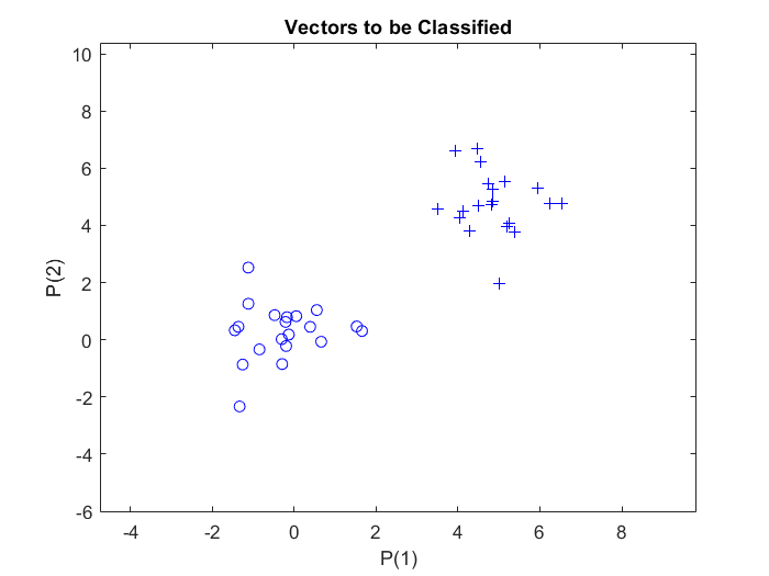
In this example, there are two clusters of data, each with $20$ samples, that belong to two classes. These clusters are defined in a two-dimensional input space. The classes are linearly separable.

Objective

To construct a perceptron for the classification of randomly defined two clusters of data.

Steps

1. Defining input and output data
2. Creating and training the perceptron
3. Plotting the decision boundary

1. Defining input and output data

At first, $20$ sample vectors of two different classes are defined randomly by using the MATLAB function randn, which generates normally distributed random numbers. An offset of $5$ is added to the samples of the second class, to have them on distinguishable distance from the samples of the first class. Each class is set as $2$-by-$20$ matrix. and combined together to generate the $2$-by-$40$ matrix $p$. Thus, matrix $p$ represent the inputs to the perceptron; normally distributed random numbers, $2$-by-$40$ ($R$-by-$Q$) matrix of $40$ input vectors of two elements each.

To assign the vectors in the matrix $p$ to one of the two classes, a second matrix, $t$, is defined to be a $1$-by-$40$ ($S$-by-$Q$) output matrix. The elements of this matrix are marked with markers, zero and one.The first $20$ elements of the $t$ matrix are assigned to zero value and the other $20$ elements are assigned to one. Thus, the output matrix $t$ consists of $40$ target vectors, each made of a single element (either zero or one).

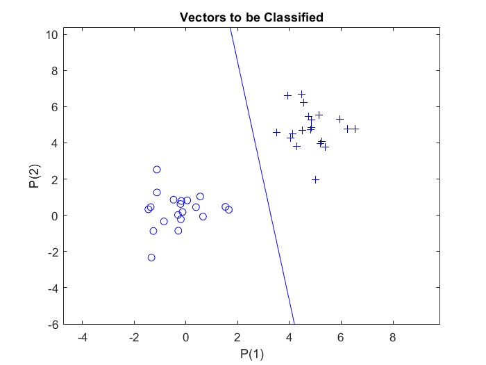
To plot the input and target vectors of the perceptron, the perceptron vector plot plotpv function is used, which takes two arguments, the first is the input matrix and the second is the target matrix. This plots column vectors in the input matrix with markers based on the output matrix.

The above code plots the samples:

2. Creating and training the perceptron

In MATLAB, a single layer perceptron is created by the command: net = perceptron;.

The perceptron uses a hard-limit transfer function, hardlim, by default.

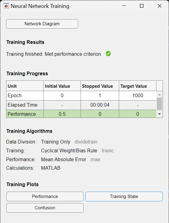
The training function for perceptron is set to trainc by default, which is cyclical order weight/bias training, and it is called by train. trainc trains a network with weight and bias learning rules with incremental updates after each presentation of an input. Inputs are presented in cyclic order. Training stops when any of these conditions is met:

• The maximum number of epochs (repetitions) is reached.
• Performance is minimized to the goal.
• The maximum amount of time is exceeded.

To measure the network performance, mean absolute error performance function, mae, is used by default. The error is calculated by subtracting the output from target. Then the mean absolute error is calculated. The goal is to minimize the performance, i.e. the error.

Resulting from the above code, the training record is displayed, showing training and performance functions and parameters, and the value of the best performance (the minimum error reached).

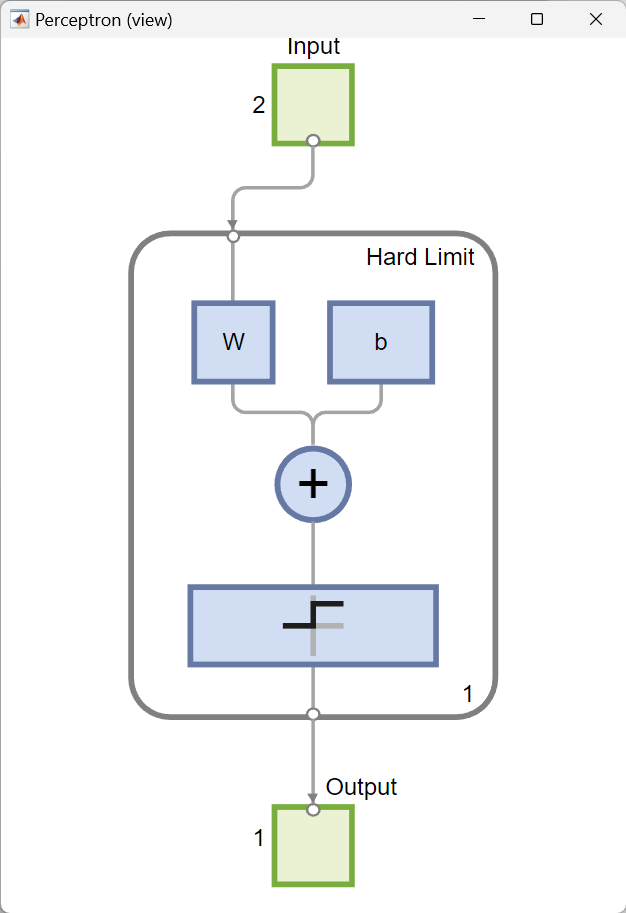
view(net) opens a window that shows the neural network (specified by net) as a graphical diagram. The numbers indicate that there are two elements in the input vectors, the network consists of one layer with a single neuron and using a hard-limit transfer function, and the output is a single element vector.

3. Plotting the decision boundary

After the network is trained, the next step is to plot the classification line on the previously plotted perceptron vector plot. This is done by plotpc function, which takes two arguments as input:

• The first one is $S$-by-$R$ weight matrix, net.iw{1,1}, which is the final weight matrix after training. \(\left\{ 1,1 \right\}\) indicates to the weights for the connection from the first input to the first layer,
• and the second argument is $S$-by-$1$ bias vector, net.b{1}, which is the final bias vector after training, for the first layer.

Here, $S$ is the number of neurons in layer and $R$ is the number of elements in input vector.

Finally, the linear decision boundary is plotted, separating data points belonging to the two class labels:

Custom Neural Networks

Problem Description and Objective

This example shows how to create and view a custom shallow neural network in MATLAB by using the network function. The network to be created is a feedforward network, consisting of two layers. It has a single input vector of six elements and an output vector (target output) of two elements. Only the first layer has a bias. An input weight connects to the first layer from the input. A layer weight connects to the second layer from the first layer. The second layer is the network output.

Steps

1. Defining the inputs and outputs
2. Defining and customizing the network (number of network subobjects)
3. Defining the topology (network subobject properties) and the transfer function
4. Configuring the network with configure
5. Training the network and calculating neuron output

1. Defining the inputs and outputs

The above code creates the input and output (target) vectors.

2. Defining and customizing the network (number of network subobjects)

To create a custom shallow neural network with one input and two layers, the next code snippet is used. The number of inputs defines how many sets of vectors the network receives as input. The size of each input (i.e., the number of elements in each input vector) is determined by the input size (in this example there is one input vector, so net.numInputs = 1 and the input size is net.inputs{1}.size = 6).

Syntax:

net = network(numInputs,numLayers,biasConnect,inputConnect,layerConnect,outputConnect)

• numInputs: Number of inputs the network receives (how many sets of vectors the network receives as input)
• numLayers: Number of layers the network has (here: two layers)
• biasConnect: numLayers-by-$1$ Boolean vector; this property defines which layers have biases ($1$ is presence and $0$ is absence) (here: the first layer has one)
• inputConnect: numLayers-by-numInputs Boolean matrix; this property defines which layers have weights coming from inputs (here: the first layer has one)
• layerConnect: numLayers-by-numLayers Boolean matrix; this property defines which layers have weights coming from other layers (here: second layer has a weight coming from first layer to second layer)
• outputConnect: $1$-by-numLayers Boolean vector; this property defines which layers generate network outputs (here: the second layer does)

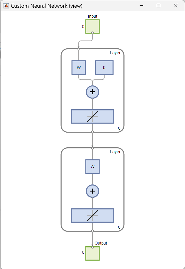
This results in a graphical diagram of the structure of the defined custom neural network:

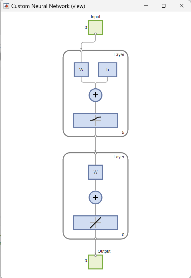
3. Defining the topology (network subobject properties) and the transfer function

The next step is to define the number of neurons in each layer. In this case, $5$ neurons are assigned to the first layer, and none to the second layer. Then, logistic sigmoid transfer function, logsig, is assigned to the first layer. To the second layer, linear transfer function, purelin, is assigned by default.

4. Configuring the network with configure

Configuration is the process of setting network input and output sizes and ranges, input preprocessing settings and output post-processing settings, and weight initialization settings to match input and target data.

The configure function configures network inputs and outputs to best match input and target data. It takes input data (here: inputs) and target data (here: outputs), and configures the network’s inputs and outputs to match. in this example, the network is configured so that the outputs of the second layer learn to match the associated target vectors.

Configuration must happen before a network’s weights and biases can be initialized. Unconfigured networks are automatically configured and initialized the first time train is called.

5. Training the network and calculating neuron output

After configuration, and before training, the network’s weights and biases are initialized by calculating the network’s output for the given input vector.

The following is the network output before training:

Initialization is followed by the training of the network with a suitable training function. In this case, Levenberg-Marquardt backpropagation (trainlm) is used as training function so that, given example input vector, the outputs of the second layer learn to match the associated target vector with minimal mean squared error (mse).

The training record is displayed:

and the output of the trained network is the desired (target) vector:

Industrial Fault Diagnosis of Connecting Rods in Compressors

Problem Description

A connecting rod in a compressor is an important factor to guarantee the reliability of a compressor. It connects the crankshaft to the piston and moves in a linear reciprocating motion along the center of the piston inside of the cylinder. It is subjected to the periodical changing load during the operation of the compressor.

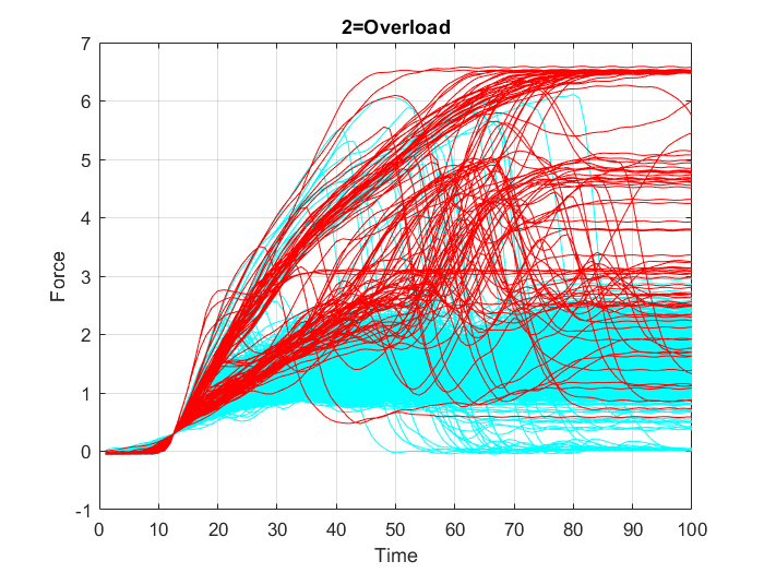
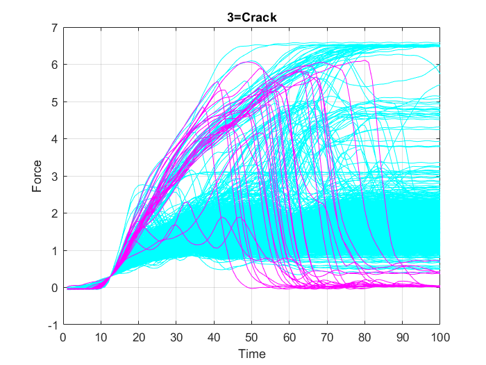
In this example, cast connecting rods are considered. A common cause of failure in these rods is structural overloading, due to enormous tensile loads caused by greater inertial forces exerted on the rods. Another cause of rod failure is the generation of micro-cracks in the metal due to concentrated stresses because of imperfections on the rod, which ultimately leads to a fracture that causes the rod to break.

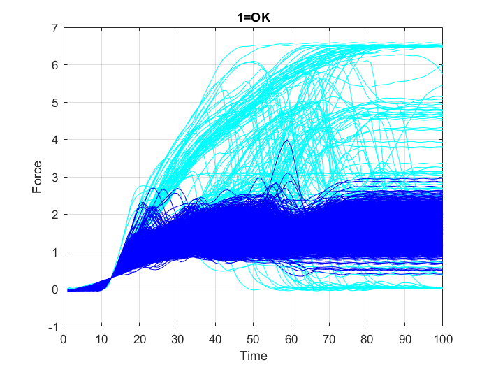
A data set from $2000$ connecting rod samples is prepared that includes the recorded periodical values, along $100$ intervals, of the changing load on each connecting rod and the respective quality condition of the rod, which in turn is divided into three classes: The first class includes the rods that remained undamaged (“OK” cases), second class includes rod failure cases due to “overload” and the third class includes rod failure cases due to “crack”.

Objective

The task is to detect, for any tested connecting rod, whether it is a defected rod (due to crack or overload) or not, from the collected data of measured periodical load values the tested rod has been carrying.

Steps

To accomplish this task a multilayer perceptron is used and the following steps are implemented to preprocess and post-process the data and to create and configure the network:

1. Loading and plotting the data
2. Preparing inputs: Data resampling
3. Defining binary output coding: 0=OK, 1=Error
4. Creating and training a multilayer perceptron
5. Post-training analysis and evaluating network performance
6. Application

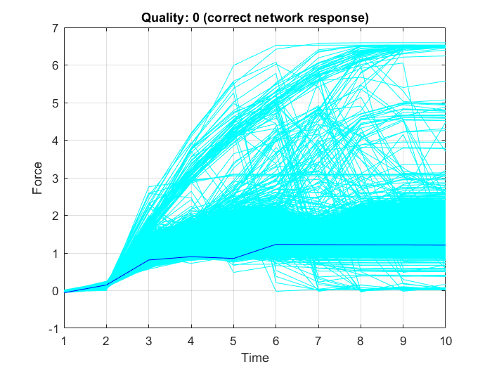
1. Loading and plotting the data

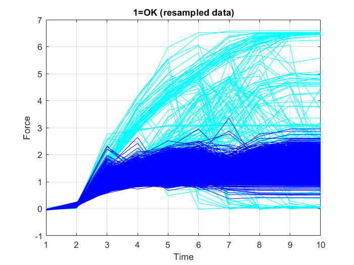
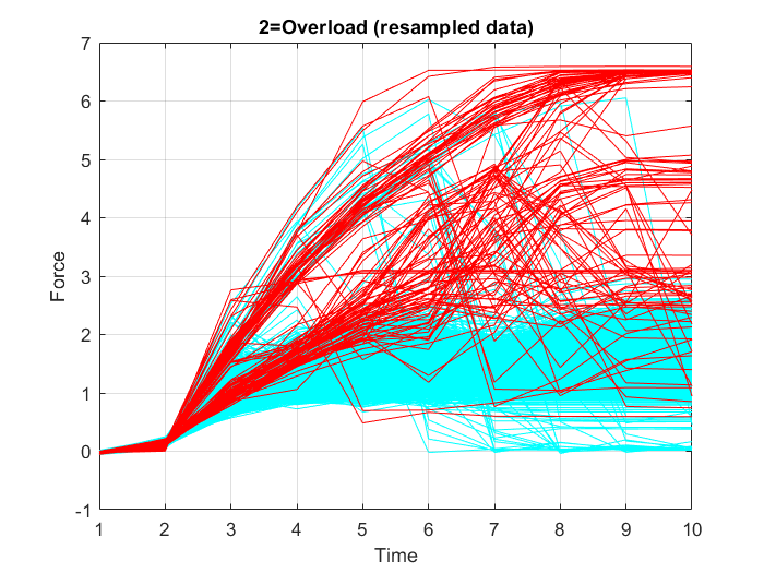
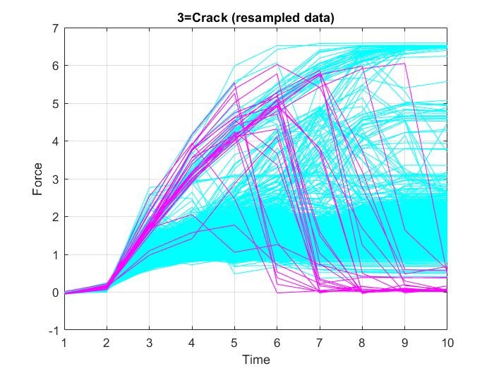
First, all variables from the data set “data.mat” are loaded into the MATLAB workspace. To check the contents of the workspace; the names, sizes, and type of all the variables in the data set, the whos function is used. Then, the data is plotted in three separate graphs, Figure 18, Figure 19 and Figure 20, in each one of them the data points belonging to only one of the three classes (“OK”, “Overload”, or “Crack”) is highlighted in some specific color, while the other points are represented in cyan color.

2. Preparing inputs: Data resampling

In this case, using the full resolution of the time series data, is not necessary. Thus, to reduce the computational resources required for model training, downsampling of the input data is carried out, which allows training on a disproportionately low subset of the majority class examples. To do this, decimation, i.e. reducing the sampling frequency by a factor of $10$, is performed on the input data, which means, keeping only every tenth sample. Figure 21, Figure 22 and Figure 23 show the graphs of the resampled data points.

3. Defining binary output coding: 0=OK, 1=Error

After resampling the input data, the target data is changed to two classes, “OK” and “Error”, by using a conditional statement, which loops through all the values of the cells inside the target data sheet one by one and returns a true or false state represented by the numbers $1$ or $0$, when the checked cell value is larger than one (“Error” class) or not (“OK” class), respectively.

4. Creating and training a multilayer perceptron

A feedforward network is created, by using MATLAB’s feedforwardnet function, to map the input and output data. It generates a feedforward network consisting of a series of layers. The first layer has a connection from the network input. Each subsequent layer has a connection from the previous layer. The final layer produces the network’s output. Size (number of neurons) of the hidden layers in the network is specified as a row vector. The length of the vector determines the number of hidden layers in the network. The input and output sizes are set to zero. The software adjusts the sizes of these during training according to the training data.

In this case, the created feedforward network consists of a single hidden layer of size $4$ (four neurons in the layer).

Then, the total data set is divided into three parts: training, validation and testing.

1. The training set is used to calculate gradients and to determine weight updates.
2. The validation set is used to stop training before overfitting occurs. The error on the validation set is monitored during the training process. The validation error normally decreases during the initial phase of training, as does the training set error. However, when the network begins to overfit the data, the error on the validation set typically begins to rise. The network weights and biases are saved at the minimum of the validation set error.
3. The test set is used to predict future performance of the network. The test set performance is the measure of network quality. If, after a network has been trained, the test set performance is not adequate, then there are usually four possible causes:
   • the network has reached a local minimum,
   • the network does not have enough neurons to fit the data,
   • the network is overfitting, or
   • the network is extrapolating.

The test set error is not used during training, but it is used to compare different models. It is also useful to plot the test set error during the training process. If the error on the test set reaches a minimum at a significantly different iteration number than the validation set error, this might indicate a poor division of the data set.

Typically, when dividing the data, approximately $70\%$ is used for training, $15\%$ for validation, and $15\%$ for testing.

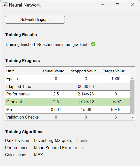
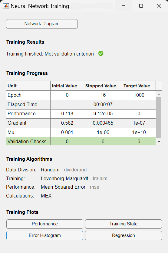
When the network weights and biases are initialized, the network is ready for training. MATLAB’s train function is used for training the network. This function uses batch training (updating the weights after the presentation of the complete data set), to differentiate it from the incremental training (updating the weights after the presentation of each single training sample), which could be carried out by MATLAB’s adapt function. The default training algorithm called by train is Levenberg-Marquardt trainlm. The training process requires a set of examples of proper network behavior,- network inputs force and target outputs target. The process of training involves tuning the values of the weights and biases of the network to optimize network performance, as defined by the network performance function. Typically one epoch of training is defined as a single presentation of all input vectors to the network. The network is then updated according to the results of all those presentations. The default performance function for feedforward networks is mean square error mse,- the average squared error between the network outputs $Y$ and the target outputs target.

During training, the progress is constantly updated in the training window. Of most interest are the performance, the magnitude of the gradient of performance and the number of validation checks. The magnitude of the gradient and the number of validation checks are used to terminate the training. The gradient will become very small as the training reaches a minimum of the performance. If the magnitude of the gradient is less than $1e-5$, the training will stop. The number of validation checks represents the number of successive iterations that the validation performance fails to decrease. If this number reaches $6$ (the default value), the training will stop.

As a result, the training record is displayed, showing training and performance functions and parameters, and the value of the best performance (the minimum error reached). In this case, the number of validation checks reached $6$ (the default value), and as a result the training stopped.

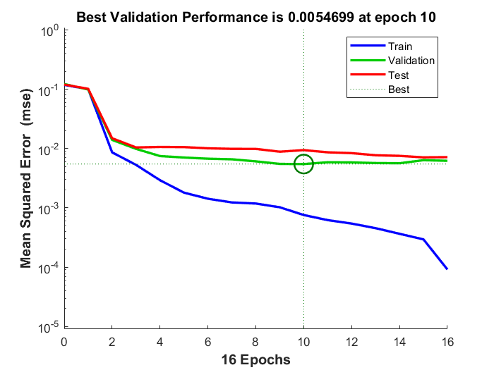
5. Post-training analysis and evaluating network performance

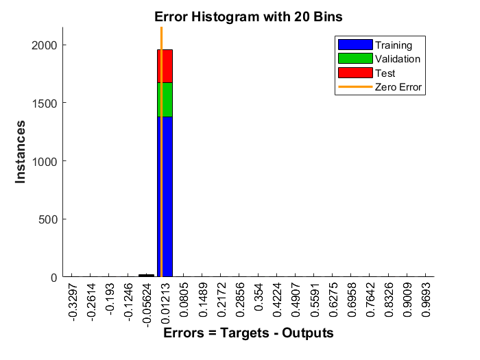
Before using a trained neural network, it should be analyzed to determine if the training was successful. There are many techniques for post-training analysis. Common ones could be obtained from the training window, where four plots are accessible: performance, training state, error histogram, and regression. The performance plot shows the value of the performance function versus the iteration number. It plots training, validation, and test performances. If there is no major problems with the training, then the error profiles for validation and test would be very similar. If the validation curve increases significantly, then it is possible that some overfitting might have occurred. The training state plot shows the progress of other training variables, such as the gradient magnitude, the number of validation checks, etc. The error histogram plot shows the distribution of the network errors. The regression plot shows a regression between network outputs and network targets. In a perfect training case, the network outputs and the targets would be exactly equal, but that is rarely the case in practice.

From the training record, performance graph, Figure 25, and error histogram, Figure 26, could be displayed. The performance graph shows that at epoch $10$ the best performance for the validation data set was reached and the training has stopped as the number of validation checks, where the validation performance fails to decrease reached $6$, and because continuing training beyond this point leads to overfitting. The performance value for the validation data set is the average of the squares of errors, and the error is the difference between the output of the network (the observed output) and the target output (the predicted output). Smaller error indicates that the outputs are very close to the target values. The error histogram shows the errors between the target values and output values after training a neural network. The more the error values are distributed closer to zero (here: the orange vertical line) the better is the model’s performance.

After training, the obtained network outputs are divided into two classes by using a threshold value and a conditional statement. $0.5$ is the natural threshold that ensures that the given probability of having $1$ is greater than the probability of having $0$. That’s why it’s the default threshold value. Output values above the threshold are labeled $1$ and values below or equal to the threshold are labeled $0$.

Finally the percentage of correct classifications could be calculated.

and it equals to $99.7\%$:

6. Application

After the network is trained and validated, the network object can be used to calculate the network response to any input; new data or from the loaded data set.

In the next code snippet a random connecting rod is selected from the data set (here:with index number $408$) and its quality is predicted correctly by the trained network (here: quality 0=”OK”), as shown in Figure 27: