Analyzing and Solving Stress and Deflection Problems, Analytically and Numerically, by Using MATLAB

PROBLEM 1: Axial Stresses and Deformations

Problem Description

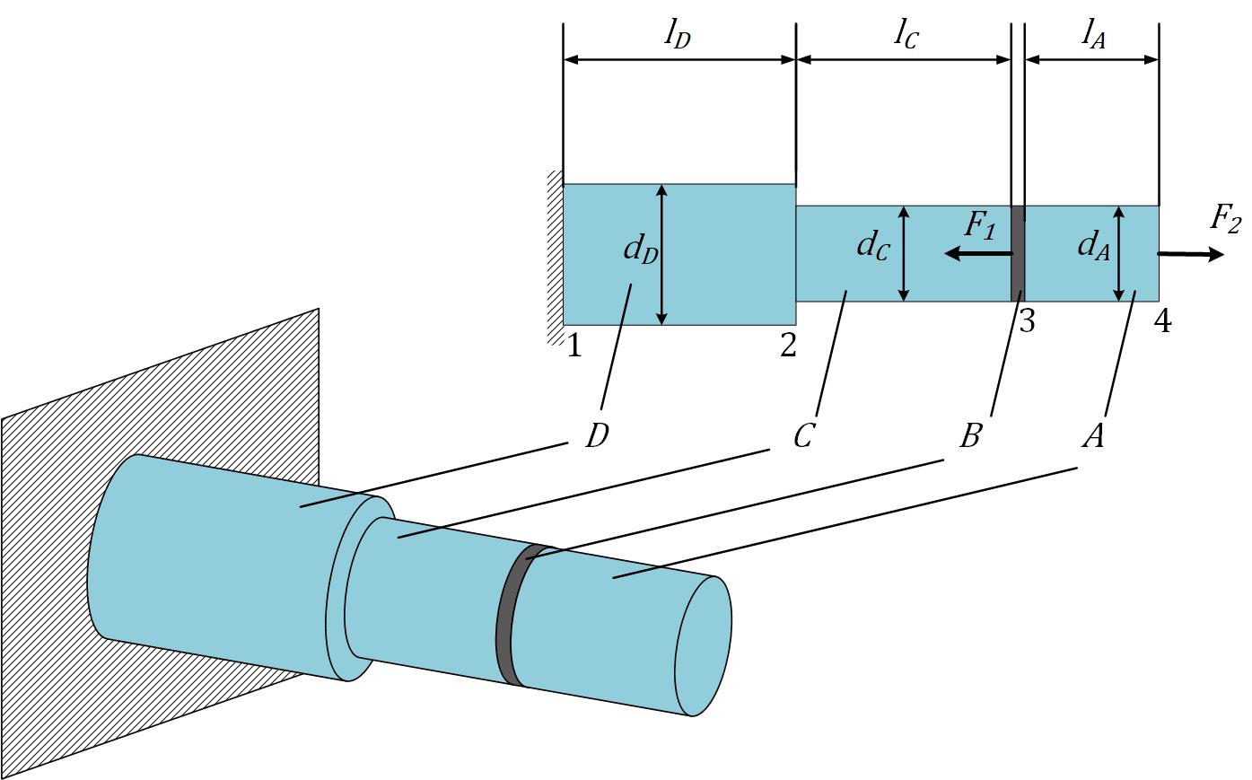
A rigid plate $\mathit{B}$ is fastened to both bars $\mathit{A}$ and $\mathit{C}$, as shown is Figure 1. Bar $\mathit{C}$ is fastened to bar $\mathit{D}$, which has its end fastened to a rigid support. The end of bar $\mathit{A}$ is free. $l_{A}$, $l_{C}$, $l_{D}$ are the lengths of the bars $\mathit{A}$, $\mathit{C}$, and $\mathit{D}$ respectively, and their diameters are $d_{A}=d$, $d_{C}=d$, and $d_{D}=1.5d$. Load $F_{1}$ is applied to the rigid plate $\mathit{B}$ $($distributed uniformly around the circumference of the rigid plate $\mathit{B})$, and load $F_{2}$ is applied at the centroid of the end cross-section of bar $\mathit{B}$.

Objectives

Determinining the axial stresses in bars $\mathit{A}$, $\mathit{C}$, and $\mathit{D}$, deformations of the bars and total deformation of the system.

For the numerical application the following values could be used:

• $F_{1} = 64000 \hspace{1pt} N$
• $F_{2} = 192000 \hspace{1pt} N$
• $d = 45 \hspace{1pt} mm$
• $l_{A} = 170 \hspace{1pt} mm$
• $l_{C} = 144.5 \hspace{1pt} mm$
• $l_{D} = 255 \hspace{1pt} mm$
• Young’s modulus $E = 21\cdot10^4 \hspace{1pt} MPa$

Solution

Analytical solution

The bar is divided into components, and the internal forces are calculated, passing sections through each component. Free-body diagrams are developed for portions of the bar, as shown in Figure 2A.

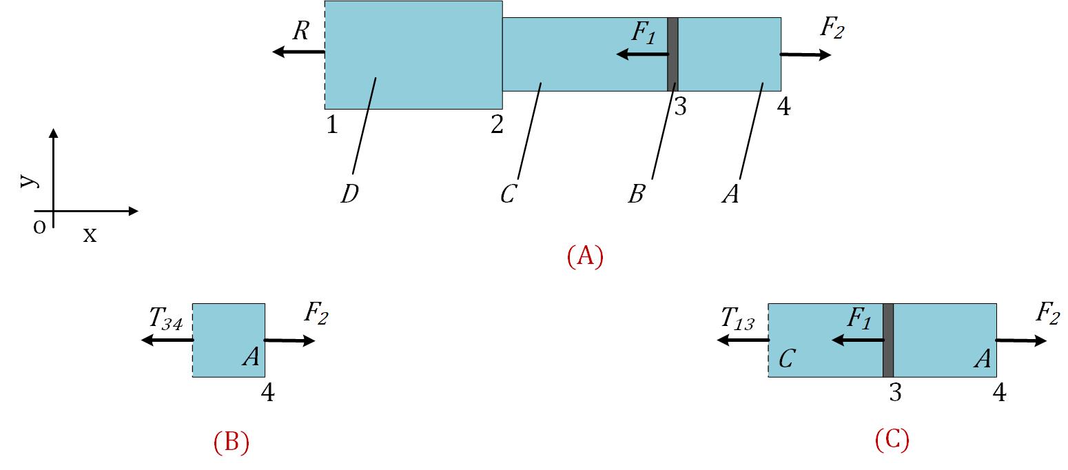
The free-body diagram of the system, namely bar $\mathit{D}$, bar $\mathit{C}$, plate $\mathit{B}$, and bar $\mathit{A}$, contains only one unknown force; the reaction force $\mathit{R}$ at the rigid support. From the equilibrium equation of the system, reaction $\mathit{R}$, or the reaction force of the rigid support on bar D, is:

• $\sum_{}^{}\mathrm{F}_{x}^{A,B,C,D}=0$
• $\Leftrightarrow R+F_{1}-F_{2}=0$
• $\Leftrightarrow R = F_{2}-F_{1}$

The MATLAB program starts with the declaration of variables as symbolic scalar variables by using syms function:

Then, the internal forces are calculated for each portion of the bar. The equilibrium equation of the free-body diagram for bar $A$, in the interval $3–4$, Figure 2B, gives the internal force $T_{34}$:

• $\sum_{}^{}\mathrm{F}_{x}^{}=0$
• $\Leftrightarrow T_{34}-F_{2}=0$
• $\Leftrightarrow T_{34}=F_{2}$

For the interval 1–3, Figure 2C, the equilibrium equation of the free-body diagram gives the internal force $T_{13}$:

• $\sum_{}^{}\mathrm{F}_{x}^{}=0$
• $\Leftrightarrow T_{13}+F_{1}-F_{2}=0$
• $\Leftrightarrow T_{13}=F_{2}-F_{1}$

The above obtained equilibrium equations are written in MATLAB as follows:

The cross-section areas of each bar $A$, $C$, and $D$ are calculated as follows:

• $A_{A}=\frac{\pi d_{A}^{2}}{4}$
• $A_{C}=\frac{\pi d_{C}^{2}}{4}$
• $A_{D}=\frac{\pi d_{D}^{2}}{4}$

In MATLAB, the cross-section areas are calculated and the results are printed with:

The axial stresses on bars $A$, $C$, $D$, namely $\sigma_{A}$, $\sigma_{C}$, and $\sigma_{D}$, are calculated using:

• $\sigma_{A}=\sigma_{34}=\frac{T_{34}}{A_{A}}=\frac{F_{2}}{A_{A}}=\frac{4F_{2}}{\pi d_{A}^{2}}$
• $\sigma_{C}=\sigma_{23}=\frac{T_{13}}{A_{C}}=\frac{F_{2}-F_{1}}{A_{C}}=\frac{4(F_{2}-F_{1})}{\pi d_{C}^{2}}$
• $\sigma_{D}=\sigma_{12}=\frac{T_{13}}{A_{D}}=\frac{F_{2}-F_{1}}{A_{D}}=\frac{4(F_{2}-F_{1})}{\pi d_{D}^{2}}$

In MATLAB, the axial stresses are calculated with:

Considering the followings:

• Hooke's law of elasticity: $\sigma=E\epsilon$, that is, for small deformations, the stress is directly proportional to the strain (that produced it),
• and the elastic strain expression: $\epsilon=\frac{\delta}{l}$, where $l$ is the bar length, $\epsilon$ is the Greek symbol used to designate strain (dimensionless), $\delta$ is the total strain (or bar elongation),

the axial displacements (i.e. the amount of elongation obtained by applying tensile load to a straight bar) of bars $C$, $D$ and the system are calculated from:

• Axial displacement of bar $D$:
$$ \delta_{12}=\frac{T_{13}l_{D}}{A_{D}E}=\frac{(F_{2}-F_{1})l_{D}}{A_{D}E} $$
• Axial displacement of bar $C$:
$$ \delta_{23}=\frac{T_{13}l_{C}}{A_{C}E}=\frac{(F_{2}-F_{1})l_{C}}{A_{C}E} $$
• Axial displacement of bars $D$ and $C$:
$$ \delta_{13}=\delta_{12}+\delta_{23}=\frac{T_{13}l_{D}}{A_{D}E} $$ $$ =\frac{(F_{2}-F_{1})l_{D}}{A_{D}E}+\frac{(F_{2}-F_{1})l_{C}}{A_{C}E} $$ $$ =\frac{(F_{2}-F_{1})}{E}\left( \frac{l_{D}}{A_{D}}+\frac{l_{C}}{A_{C}} \right) $$
• Axial displacement of bar $A$:
$$ \delta_{34}=\frac{T_{34}l_{A}}{A_{A}E}=\frac{F_{2}l_{A}}{A_{A}E} $$
• Total axial displacement of the system:
$$ \delta_{14}=\delta_{13}+\delta_{34} $$ $$ =\frac{(F_{2}-F_{1})}{E}\left( \frac{l_{D}}{A_{D}}+\frac{l_{C}}{A_{C}} \right) +\frac{F_{2}l_{A}}{A_{A}E} $$

In MATLAB, the axial displacement of the bars and system are calculated with:

Numerical solution

To numerically calculate the axial stress and displacements, first the numerical data, given in the problem description, is introduced into the MATLAB code and then the symbolic variables are substituted with the numerical data. For the first part, two cell arrays are introduced. The string values (the symbolic variables) of the numerical data are put into cell array lists and their numerical values in cell array listn. For the second part, MATLAB’s symbolic substitution function subs is used to replace the symbolic variables in lists with their respective values from the listn, then they are displayed on the screen.

In a similar way the numerical values of each bar diameter are displayed and values of cross-section are calculated by using MATLAB’s eval function then displayed:

The numerical values of each bar length are expressed in MATLAB by:

Finally, the numerical values of the axial stresses are calculated and displayed in MATLAB with:

and the results are:

The numerical values of the axial displacement of the bars and the system are calculated in MATLAB with:

and the results are:

Diagrams

The force, stress and displacement diagrams (Figure 3) are obtained using the following MATLAB code:

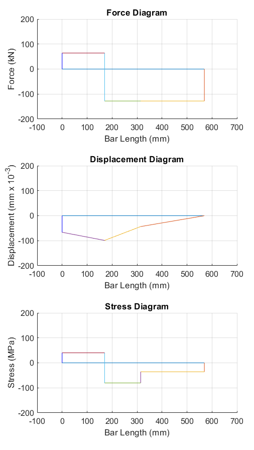
Three MATLAB functions are used to obtain the diagrams, namely: ForceDdraw, StressDdraw and DisplacementDdraw, by using the line function, which takes two input arguments. This function plots lines in the current axes by connecting the data in both input vectors (or matrices). In this case, both input arguments are vectors, where the first vector is the $x$-coordinates and the second vector the $y$-coordinates. Because both input vectors are of equal length, the line function plots a single line each time it is used. The codes for the three MATLAB functions are as follows:

• The MATLAB function ForceDdraw is:
function []=ForceDdraw(F1A,F2A,l1,l2,l3,l4)
xlabel('Bar Length (mm)'), ylabel('Force (kN)')
title('Force Diagram')
hold on; grid on
axis equal; axis on
axis([-100 700 -200 200 ])
hold on;
scale_F=1000;
hold on
l=line([0 (l1+l2+l3)], [0 0]);
l=line([(l1+l2+l3) (l1+l2+l3)], [0 F1A/scale_F]);
l=line([(l1+l2+l3) (l1+l2+l3)-(l3)],...
[F1A/scale_F F1A/scale_F]);
l=line([(l1+l2+l3)-l3 (l1+l2+l3)-(l3)],...
[F1A/scale_F F1A/scale_F]);
l=line([(l1+l2+l3)-l3 (l1+l2+l3)-(l2+l3)],...
[F1A/scale_F F1A/scale_F]);
l=line([(l1+l2+l3)-(l2+l3) (l1+l2+l3)-(l2+l3)],...
[F1A/scale_F F2A/scale_F]);
l=line([0 (l1+l2+l3)-(l2+l3)],...
[F2A/scale_F F2A/scale_F]);
l=line([0 0], [F2A/scale_F 0]);
set(l,'Color','blue');
end


• The MATLAB function StressDdraw is:
function []=StressDdraw(sigma1,sigma2,sigma3,l1,l2,l3)
xlabel('Bar Length (mm)'), ylabel('Stress (MPa)')
title('Stress Diagram')
hold on; grid on
axis equal; axis on
axis([-100 700 -200 200])
hold on;
scale_S=1;
hold on
l=line([0 (l1+l2+l3)],[0 0]);
l=line([(l1+l2+l3) (l1+l2+l3)],[0 sigma3]);
l=line([(l1+l2+l3) (l1+l2+l3)-(l3)],...
[sigma3/scale_S sigma3/scale_S]);
l=line([(l1+l2+l3)-(l3) (l1+l2+l3)-(l3)],...
[sigma3/scale_S sigma2/scale_S]);
l=line([(l1+l2+l3)-(l3) (l1+l2+l3)-(l2+l3)],...
[sigma2/scale_S sigma2/scale_S]);
l=line([(l1+l2+l3)-(l2+l3) (l1+l2+l3)-(l2+l3)],...
[sigma2/scale_S sigma1/scale_S]);
l=line([0 (l1+l2+l3)-(l2+l3)],...
[sigma1/scale_S sigma1/scale_S]);
l=line([0 0],[sigma1/scale_S 0]);
set(l,'Color','blue');
end


• The MATLAB function DisplacementDdraw is:
function []=DisplacementDdraw(delta1,delta2,delta3,l1,l2,l3)
xlabel('Bar Length (mm)'), ylabel('Displacement (mm x 10^{-3})')
title('Displacement Diagram')
hold on; grid on
axis equal; axis on
axis([-100 700 -200 200])
hold on;
scale_D=10^(-3);
hold on
l=line([0 (l1+l2+l3)], [0 0]);
l=line([(l1+l2+l3) (l1+l2+l3)-(l3)],...
[0 delta3/scale_D]);
l=line([(l1+l2+l3)-(l3) (l1+l2+l3)-(l2+l3)],...
[delta3/scale_D delta2/scale_D]);
l=line([(l1+l2+l3)-(l2+l3) (l1+l2+l3)-(l1+l2+l3)],...
[delta2/scale_D delta1/scale_D]);
l=line([0 0], [delta1/scale_D 0]);
set(l,'Color','blue');
end

PROBLEM 2: Bending and Shear Stresses

Problem Description

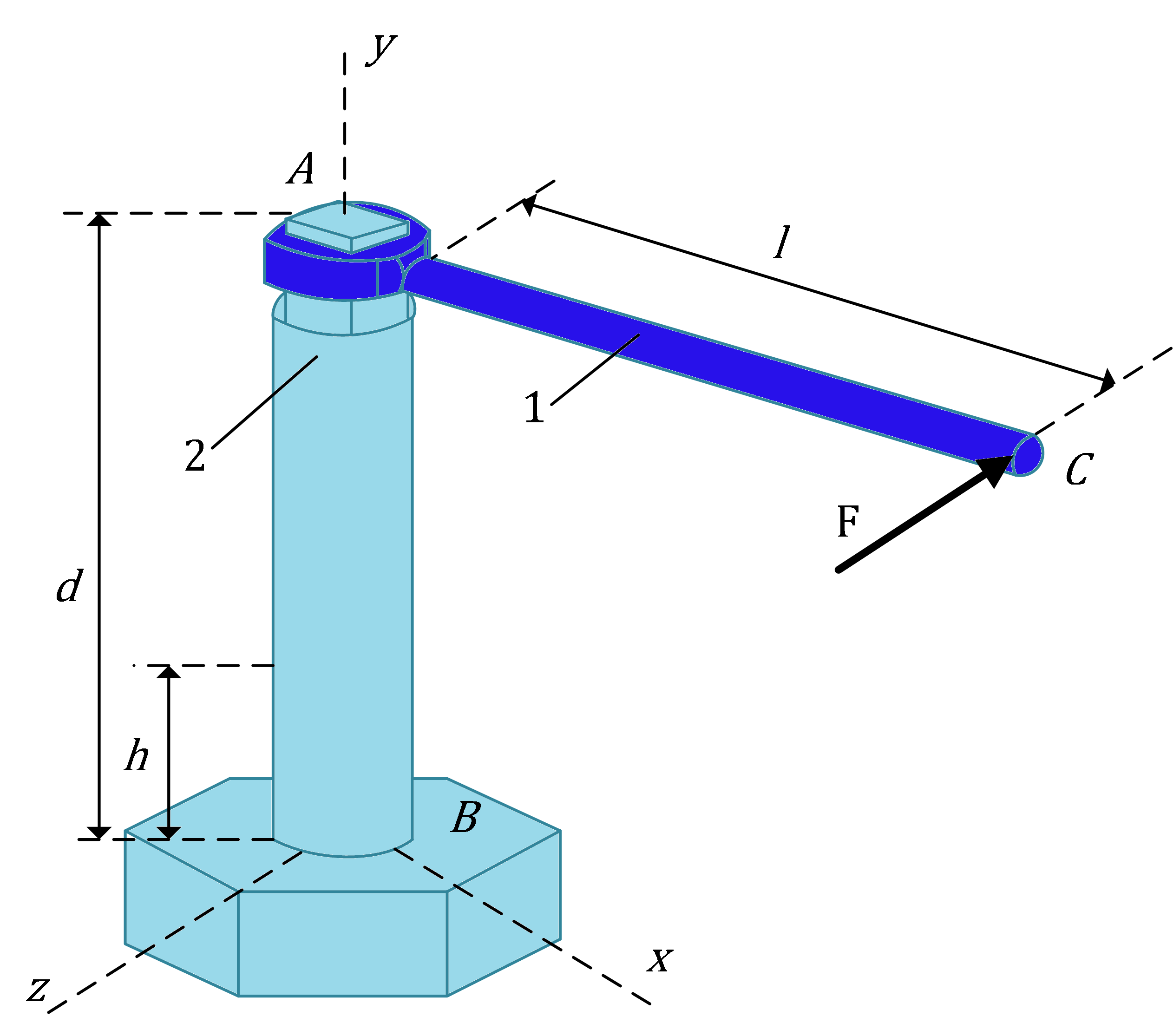
A Lever $(1)$ with length $AC = l$ is fit on a tapered lever bar $(2)$ denoted by $AB$. The lever is subjected at its end to a horizontal force $F$, as shown in Figure 4. The lever bar has radius $r$ and length $d$.

For the numerical application the following values could be used:

• $F = 250 \hspace{1pt} N$
• $d = 200 \hspace{1pt} mm$
• $l = 250 \hspace{1pt} mm$
• $h = 50 \hspace{1pt} mm$
• $r = 9 \hspace{1pt} mm$

Objectives

• Determining the normal and shear stresses of an element located on the free surface of lever bar $(2)$ at a distance $h$ from the hexagonal base (the element is parallel to the plane determined by the axes $x$, $y$).
• Constructing the Mohr’s circle and determining the principal planes and stresses.

Solution

The force $F$ causes bending moment (pure bending) and a torque (twisting moment) on the bar. Thus, bending induces bending stresses, which are normal stresses, and shear stresses distributed over the cross section.

The normal and shear stresses of a general element parallel to the plane determined by the axes $x$, $y$ located at a distance $h$ from the hexagonal base are $\sigma_{y}$ and $\tau_{yz}$ respectively.

Bending Stresses

$\sigma_{y}$ is the bending stress distribution over the bending height, for the case of pure bending:

The different subscripts express that the bending stress in $y$ direction is distributed over the bending height defined here by the $z$ coordinate, and $x$ is the neutral axis.

• $M_{b,x}$ is the bending moment, it equals to:

• $I_{x}$ is the area moment of inertia (also referred to as second moment of area). It is a geometrical property of a shape describing the distribution of points around an axis. In classical mechanics it is used as a measure of a body’s resistance against bending. For a circular cross-section it equals to:

• The bending height $z$ is the perpendicular distance of a point along the cross-section of the bar from its neutral axis, and when calculating the maximum bending stress then $z$ equals to $r$, because it is where the bending stress is at its maximum value along the cross-section.

The bending stress equation shows that the bending stress increases linearly as the bending moment and the distance from the neutral axis increase, and it decreases as the area moment of inertia increases. The maximum stress occurs at the fibers furthest from the neutral axis. The term $\frac{z}{I_{x}}$ depends only on the geometry of the cross-section.

Thus, the maximum bending stress equals to:

Shear Stresses

Torsion is the twisting of an object, caused by a moment acting about the object’s longitudinal axis. A moment which tends to cause twisting is called torque.

Torsion generates shear stresses and strains within the bar. Both shear strains and shear stresses increase linearly with the distance from the center of the cross-section, with the maximum shear stress and shear strain occurring on the outer surface.

The maximum shear stress due to torsion for a circular cross-section is given by the equation:

This means, shear stress is a function of

• the torque $T_{y}$, here: around the $y$ axis,
• the distance from the center of the cross-section, here: equal to $r$; the distance to the edge,
• and the polar moment of inertia $J_{p}$.

For a circular cross section, the polar moment of inertia is:

The torque $T_{y}= F \cdot l$.

Stress Transformation and Mohr’s Circle

Considering a 2D stress element, corresponding to a state of plane stress (for example the $xy$-plane), the four faces of the element are under normal stresses and shear stresses. Supposing that this element is cut by an oblique plane with a normal at an arbitrary angle $\phi$ counterclockwise from the $x$ axis, then the values of the normal and shear stresses could be calculated by using the stress transformation equations:

• $\sigma = \frac{\sigma_{x}+\sigma_{y}}{2}+\frac{\sigma_{x}-\sigma_{y}}{2}\cdot cos(2\phi)+\tau_{xy}\cdot sin(2\phi)$
• $\tau = \frac{\sigma_{x}-\sigma_{y}}{2}\cdot sin(2\phi)+\tau_{xy}\cdot cos(2\phi)$

Differentiating the first equation with respect to $\phi$ and setting the result equal to zero maximizes $\sigma$ and gives:

• $tan(2\phi)=\frac{2\tau_{xy}}{\sigma_{x}-\sigma_{y}}$

This equation defines two particular values for the angle $2\phi$, one of which defines the maximum normal stress $\sigma_{1}$ and the other, the minimum normal stress $\sigma_{2}$. These two stresses are called the principal stresses, and their corresponding directions, the principal directions. The angle between the two principal directions is $90°$. This equation can be obtained from the second equation of the stress transformation equations by setting $\tau =0$, meaning that the perpendicular surfaces containing principal stresses have zero shear stresses.

An important thing to note is that angles in Mohr’s circle are doubled compared to the stress element’s rotation angle. For example, by observing Mohr’s circle, there is a $180$ degree angle between the minimum and maximum principal stresses, whereas on the stress element the angle is $90$ degrees. This is why $2\phi$ notation is used on Mohr’s circle. $\phi$ is the angle of rotation of the stress element, and $2\phi$ is the corresponding angle on Mohr’s circle.

Formulas for the two principal stresses can be obtained by substituting the angle $2\phi$ in the first stress transformation equation:

• $\sigma_{1}, \sigma_{2} =\frac{\sigma_{x}+\sigma_{y}}{2}\pm \sqrt{({\frac{\sigma_{x}-\sigma_{y}}{2})^{2}}+\tau_{xy}^{2}}$

In a similar manner, by differentiating the second stress transformation equation with respect to $\phi$ and setting the result equal to zero gives:

• $tan(2\phi)=-\frac{\sigma_{x}-\sigma_{y}}{2\tau_{xy}}$

This defines the two values of $2\phi$ at which the shear stress $\tau$ reaches an extreme value (not maximum). The angle between the two surfaces containing the maximum shear stresses is $90°$.

Formulas for the two extreme-value shear stresses are obtained by substituting the angle $2\phi$ in the second stress transformation equation:

• $\tau_{1}, \tau_{2} =\pm \sqrt{({\frac{\sigma_{x}-\sigma_{y}}{2})^{2}}+\tau_{xy}^{2}}$

Analytical solution

The MATLAB program starts with the declaration of variables as symbolic scalar variables by using syms function:

Then, the normal and shear stresses are calculated in MATLAB with:

This results in the following output:

Then the element orientation and principal stresses are calculated in MATLAB with:

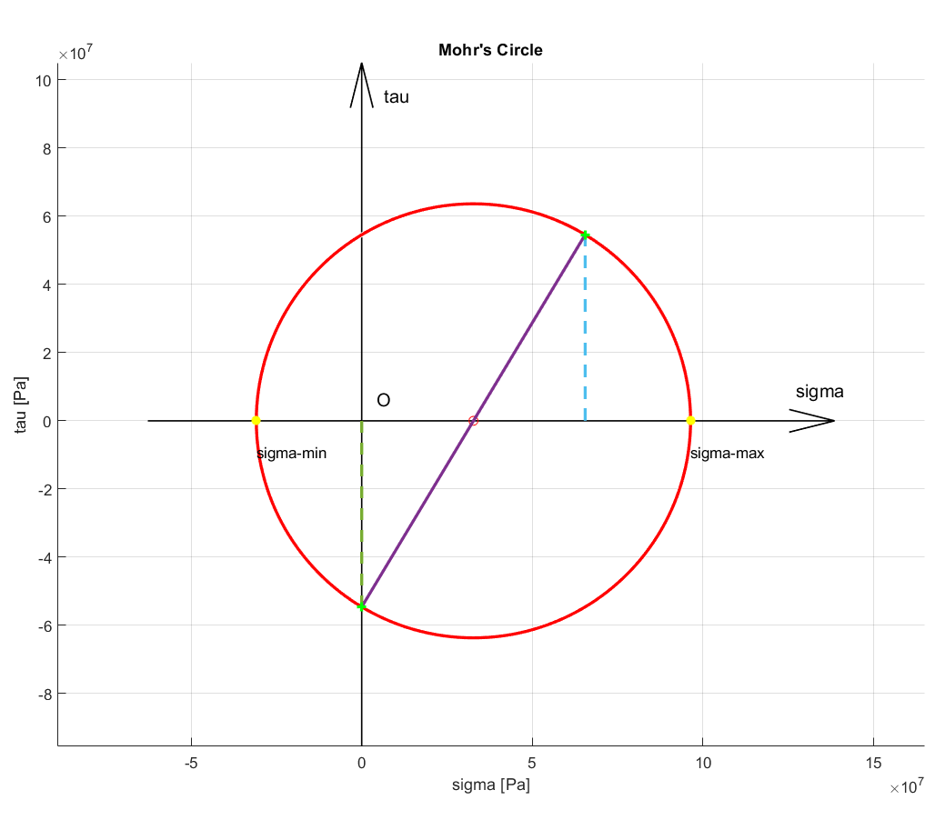
For this, the user created function mohr2D(sigma_x,sigma_y,tau,phi) is required, to calculate:

• the maximum normal stress $\sigma_{1}$ (sigma_max) and minimum normal stress $\sigma_{2}$ (sigma_min). Mohr's circle crosses the horizontal axis at these two locations, as the shear stress is zero. These two values can also be calculated by taking the $x$ coordinate of the circle's center, and adding or subtracting the circle radius
• the radius (radius) of the Mohr's circle, which equals to $\sqrt{({\frac{\sigma_{x}-\sigma_{y}}{2})^{2}}+\tau_{xy}^{2}}$, which is also the value of the maximum shear stress
• the center (center_circle) of the Mohr's circle, which is at $(\frac{\sigma_{x}+\sigma_{y}}{2},0)$
• the angle $\phi$, named phi in the code, between the original stress element and the principal planes. $tan(2\phi)$ is named phi_p in the code.

This function is created by the following code:

And the output of this code is:

Numerical solution

For numerical calculations, the numerical data for the applied force $F$, the length of the lever $l$, the lever bar’s radius $r$ and length $d$, and the distance $h$ of the element on the lever bar are introduced in MATLAB as input with the code:

The numerical values for the equivalent force system; torque $T_{y}$, force $F$ and bending moment $M_{b,x}$, is calculated and printed in MATLAB with:

resulting in:

The numerical values for the stress orientation and principal stresses are calculated and displayed in MATLAB with:

resulting in:

Graphical Representation

The graphical representation of the Mohr’s circle (Figure 5) is obtained in MATLAB by calling the user created function mohr2Ddraw:

The code for the mohr2Ddraw function is: