Lane Lines Detection using Real-Time Machine Vision for Seeing Vehicles
Line detection plays a crucial role in machine vision applications, as in automated detection of lane lines in autonomous (self-driving) seeing vehicles and mobile machines. The task being to piece together a pipeline to detect line segments in driving lanes from an image of the road or path then applying the working pipeline on a video stream.
OBJECTIVES
Building a program in Python to identify road or path lanes in an image, then applying this pipeline to a video stream, recorded by a camera placed on a vehicle, to identify road lane boundaries in it.
AQUIRED SKILLS
- Computer Vision techniques via Python used to identify lane boundaries in both images and video streams.
- Using the OpenCV, NumPy and Matplotlib libraries.
- Image processing by using image arithmetic.
- Filtering out image noise and smoothing with Gaussian filter.
- Using edge detection algorithms to identify boundaries of objects, in particular, the Canny edge detector.
- Creating an edge detection algorithm.
- Feature extraction by using the Hough transform technique.
- Optimization of extracted features by averaging.
STEPS
The lane detection pipeline described here has the following structure:
- 1. Loading the Image
- 2. Edge Detection
- 3. Region of Interest
- 4. Hough Transform
- 5. Optimization
- 6. Identifying Lane Lines in a Video
1. Loading the Image
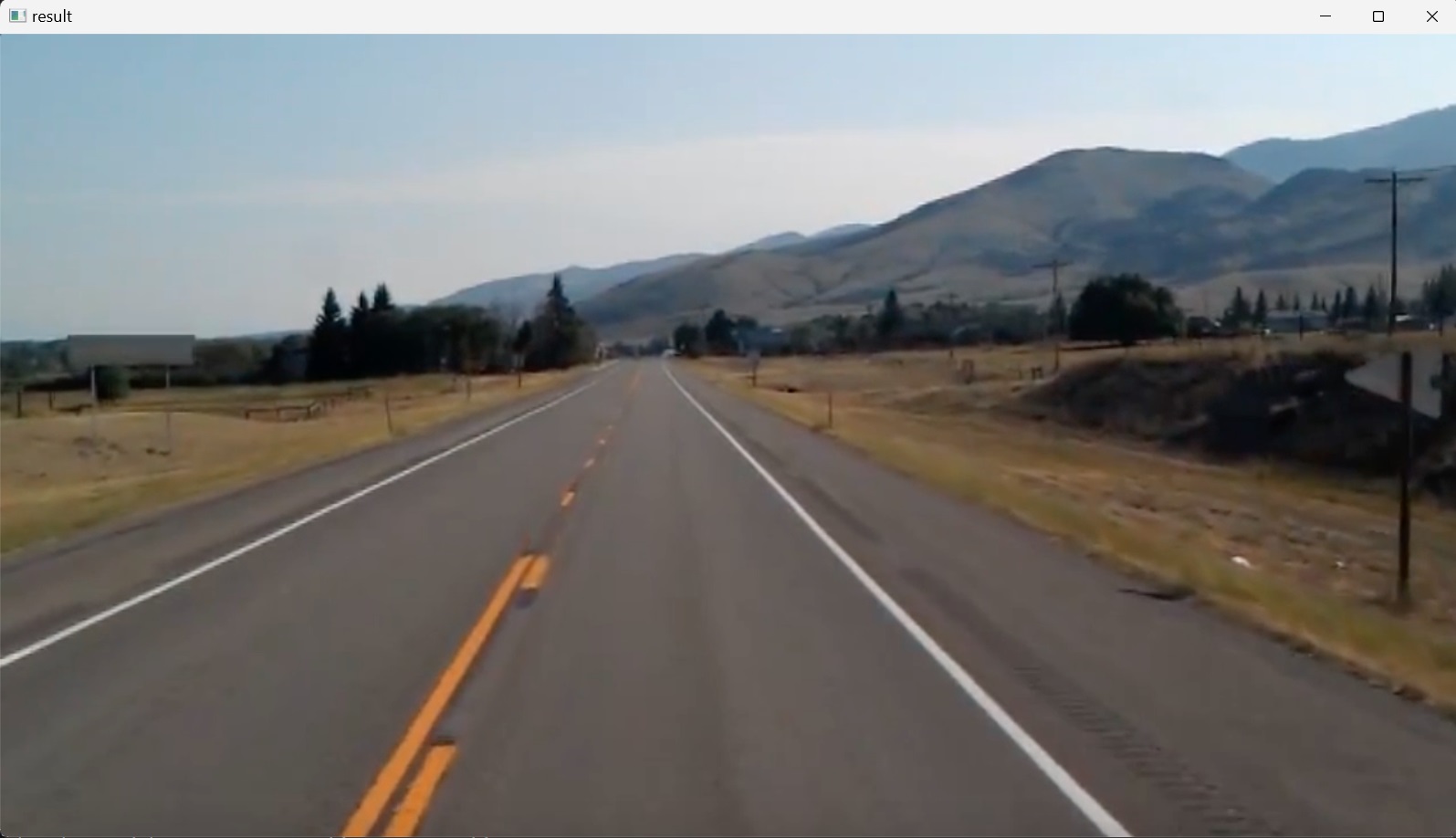
In this step a test image is loaded into the project by importing the OpenCV library and accessing its function imread(), which reads the test image from a folder and returns it as a multidimensional NumPy array containing the relative intensities of each pixel in the image. Then the test image is rendered with the imshow() function, which takes two arguments; the first one is the name of the window (here: “result”) in which the image1 (Figure 1), the second argument, will be displayed. This is followed by the waitKey() function, which specifies a duration of milliseconds to display the image; with $0$ value indicating a infinite display until any keyboard button is pressed.
import cv2

image1 = cv2.imread('test_image.jpg')
cv2.imshow("result", image1)
cv2.waitKey(0)
2. Edge Detection
Edge detection is one of the fundamental steps in image processing, image analysis, image pattern recognition, and computer vision techniques.
Edges are sudden discontinuities in an image. Edge locations are identified in an image from the intensity profile of this image along a row or column.
Thinking of an image as a grid, each square in the grid contains a pixel (short for picture element), thus an image is a tiling (an array) of pixels.
A digital color image can be represented as an array of pixels (grid of pixels) where each pixel has three channels and is represented as a $1\times3$ vector, usually of integer values, representing an RGB data value (Red, Green, Blue), which is considered to give the color, the RGB intensities (the amount of light) that appears in a given location in the image. The minimum intensity value for a basic color is $0$. The maximum intensity is $255$. This means that Each pixel’s color sample has three numerical RGB components (Red, Green, Blue) to represent the color of that tiny pixel area. These three RGB components are three $8$-bit numbers for each pixel. There are actually $256$ (i.e. $8$-bit format; $2^8=256$) different amounts of intensity for each basic color. Since the three colors have integer values from $0$ to $255$, there are a total of $256\times256\times256 = 16,777,216$ combinations or color choices. Black is an RGB value of $(0, 0, 0)$ and White is $(255, 255, 255)$. Gray, however, has equal RGB values. Thus, $(220, 220, 220)$ is a light gray (near white), and $(40,40,40)$ is a dark gray (near black).
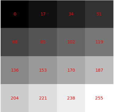
Since gray has equal values in RGB, black-and-white grayscale images only use one byte of $8$-bit data per pixel instead of three. Each pixel has a value between $0$ and $255$, where zero represents ‘no intensity’ or ‘black’ and $255$ represents ‘maximum intensity’ or ‘white’. The values progress gradually from $0$ to $255$ representing $256$ shades of gray; darker to lighter. This is why in image processing, color images are converted into grayscale to perform edge detection as this helps in simplifying algorithms and eliminates the complexities related to computational requirements.
Figure 2 shows a grayscale image, divided into a matrix of square shapes, where each square consists of pixels in some intensity value. The intensity values are displayed in red. To generate this, the following Python code was used:
import numpy as np
import matplotlib.pyplot as plt


array = np.array([[0, 17, 34, 51],
                  [68, 85, 102, 119],
                  [136, 153, 170, 187],
                  [204, 221, 238, 255]])
plt.imshow(array, cmap = 'gray')
for i in range(array.shape[0]):
    for j in range(array.shape[1]):
        plt.text(j,i, str(array[i,j]),color='r', ha='center', va='center')
plt.axis("off")
plt.show()
Here, after defining an array of values, the array was plotted to display a grayscale image, where the colormap was set up by using the matplotlib parameter cmap='gray'.
Edge detection methods rely on the computation of image gradients, which is the directional change in image intensity. Regions in an image that look like edges are detected by measuring the gradient, i.e. the change in intensity values, at each pixel of the input image, in a given direction. After applying an edge detector on the original image, sharp changes in image brightness are detected. In the resulting gradient image the discontinuities in image brightness are represented by set of connected curves and lines that indicate the boundaries of objects. Discontinuities in image brightness correspond to discontinuities in depth, in surface orientation, changes in material properties and variations in scene illumination.
There are many edge-detection methods, including Canny, Sobel, Laplacian, and Prewitt. These can be grouped into two categories, gradient and Laplacian. The gradient method (Canny, Sobel) detects the edges by looking for the maximum and minimum in the first derivative of the image. The Laplacian method (Laplacian, Prewitt) searches for zero-crossings in the second derivative of the image to find edges. However, the Canny edge detector is arguably the most commonly used edge detector in the field as its algorithm is one of the most strictly defined methods that provides good and reliable detection.
Grayscale conversion
Color edge detection is used only in some special cases because its calculation requirements are three times greater than in the case of grayscale image and most of the edges are about the same in gray value and in color images.
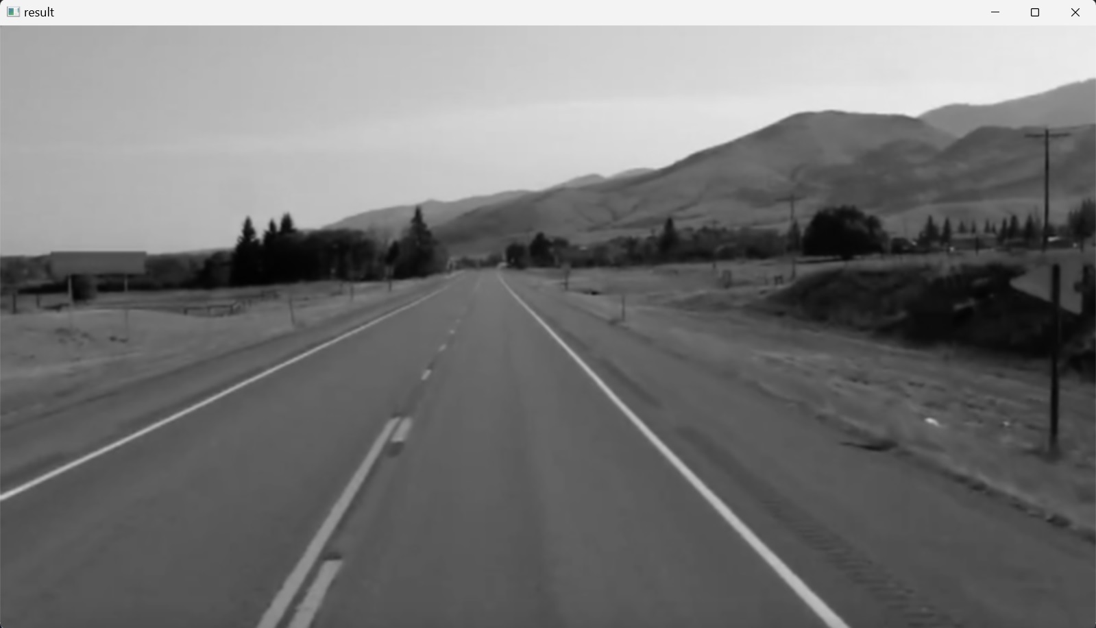
Before going into the Canny edge-detector algorithm, some preprocessing steps are taken, starting with importing the OpenCV and NumPy libraries, reading in the image, using the imread() function in OpenCV, copying the loaded image array into a new variable with the np.copy() function of NumPy, to not alter the original image. These are followed by reading in the color image as a grayscale image with the Color Space Conversions function cvtColor() of OpenCV, used for converting the color space of an image. It takes an input image in one color space and transforms it into another color space; in this case, converting from RGB to Grayscale, as shown in the next code.
OpenCV uses BGR image format (color space). When reading an RGB image using OpenCV it interprets the image in BGR format by default, thus, cv2.COLOR_BGR2GRAY is used as the color space conversion code.
import cv2
import numpy as np

image1 = cv2.imread('test_image.jpg')
lane_image = np.copy(image1)
gray_image = cv2.cvtColor(lane_image, cv2.COLOR_BGR2GRAY)
cv2.imshow("result", gray_image)
cv2.waitKey(0)
The result is shown in Figure 3.

To illustrate quickly the above mentioned difference between RGB and BGR the following code reads an image by using the imread() method of OpenCV and displays it using the Matplotlib package, as well as OpenCV’s imshow() method.
import cv2
import matplotlib.pyplot as plt

image2 = cv2.imread('museum_im_schloss.jpg')

# Using OpenCV
cv2.imshow('Displaying image using OpenCV', image2)
cv2.waitKey(0)

# Using Matplotlib
plt.imshow(image2)
plt.title('Displaying image using Matplotlib')
plt.show()
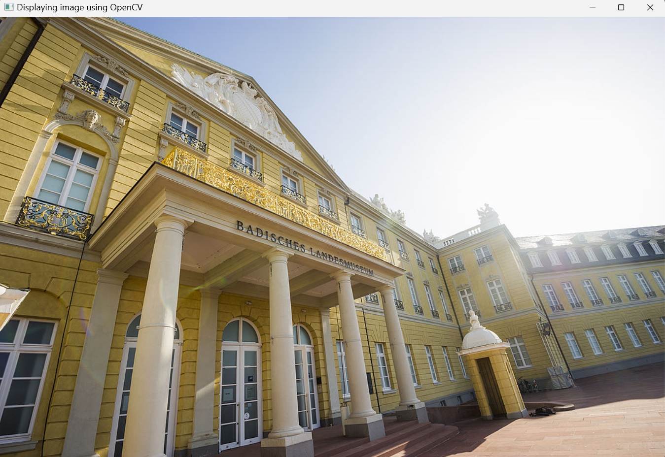
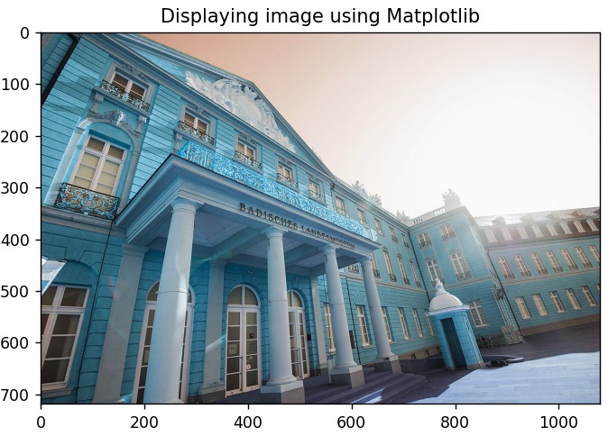
The reason for the difference in colors between the two displays is that OpenCV reads and displays the image in BGR rather than RGB order. Matplotlib, on the other hand, uses the RGB color format and thus, requires that the BGR image is converted to RGB first, to display it correctly.
However, back to the grayscale conversion in OpenCV, converting an RGB image to grayscale is not straightforward. This is realized through the method of color mode expression. $R_{i}$, $G_{i}$, and $B_{i}$ represent the three primary color values of each pixel, respectively, and the gray data $C_{i}$ of each pixel are obtained by calculating the mean value of its RGB data.
In human vision, however, eyes are more sensitive and thus perceive more green, less sensitive to red and the least sensitive to blue. Therefore, weights of the linear weighted average are defined to compensate nonuniformity of the sensitivity and following this, different weights are assigned to the three colors. The weight values of the general R, G, and B components are $0.299$, $0.587$, and $0.114$, respectively.
Thus, when converting to grayscale, each of the RGB channels is not weighted uniformly, like this:
\[C_{i} = 0.33 \times R_{i} + 0.33 \times G_{i} + 0.33 \times B_{i}\]Rather, each channel is weighted differently to account for human vision. The conversion model can be expressed:
\[C_{i} = 0.299 \times R_{i} + 0.587 \times G_{i} + 0.114 \times B_{i}\]Canny edge-detection algorithm
The process of Canny edge-detection algorithm can be broken down to five different steps:
- Noise reduction by smoothing the image with Gaussian filter
- Finding the intensity gradients of pixels in the image by using Sobel filter
- Applying gradient magnitude thresholding or Non-maximum suppression to get rid of false edges
- Applying double threshold to determine potential edges
- Edge tracking by hysteresis: Finalizing the detection of edges by suppressing all the other edges that are weak and not connected to strong edges.
Step 1: Smoothing with Gaussian filter
There are two main types of image processing: image filtering and image warping. Image filtering changes the pixel values of an image, altering the color intensities, without changing the pixel positions, while image warping changes the pixel positions of an image without changing the colors.
After reading in the image, the next step is to blur it, using the GaussianBlur() function. This is done to reduce the noise in the image, as most edge-detection algorithms are sensitive to noise, and to smoothen the intensity variation near the edges, making it easier to identify the predominant edge structure within the image.
Mathematically, applying a Gaussian blur to an image is the same as convolving the image with a Gaussian function (which also expresses the normal distribution in statistics). Values from this distribution are used to build a convolution matrix which is applied to the original image. Each pixel’s new value is set to a weighted average of that pixel’s neighborhood. The original pixel’s value receives the heaviest weight (having the highest Gaussian value) and neighboring pixels receive smaller weights as their distance to the original pixel increases. This results in a blur that preserves boundaries and edges better than other, more uniform blurring filters. Convolution is done by using a kernel and iterating through an input image to create an output image.
In edge detection, noise can cause false edges to appear in the result. Using a Gaussian blur filter before edge detection aims to reduce this level of noise in the image, which improves the result of the used edge-detection algorithm.
The following line of code blur = cv2.GaussianBlur(gray,(5,5),0) applys a Gaussian blur on the grayscale image gray_image with a $5\times5$ kernel and zero deviation, and returns a new image called blur_image. The size of the kernel varies depending on specific situations. The larger the size is, the lower the detector’s sensitivity to noise. Additionally, the localization error to detect the edge will slightly increase with the increase of the Gaussian filter kernel size. A $5\times5$ is a good size for most cases.
The following Python code applies Gaussian blur to the grayscale path or road image and displays the output (Figure 6).
import cv2
import numpy as np

image1 = cv2.imread('test_image.jpg')
lane_image = np.copy(image1)
gray_image = cv2.cvtColor(lane_image, cv2.COLOR_BGR2GRAY)
blur_image = cv2.GaussianBlur(gray_image,(5,5),0)
cv2.imshow("result", blur_image)
cv2.waitKey(0)
After grayscale conversion and blurring are done, Canny edge detector is applied now directly to the blurred image by calling the function cv2.Canny() in the code.
Step 2: Calculating the intensity gradients
An image can be considered to be an array of samples of some continuous function of image intensity. An edge in an image may point in a variety of directions, so the Canny algorithm uses the concept of derivatives, typically the Sobel operator, to determine both the gradient magnitude and orientation for each pixel. The gradient magnitude indicates the strength of the intensity change; a small derivative is a small change in intensity, whereas a big derivative is a big change, while the gradient orientation specifies the direction of the steepest change.
The Sobel operator is an edge detection operator used to find the gradient, or the rate of change, in both the horizontal (from left to right) and vertical (from top to bottom) directions of an image. It returns a value for the first derivative of the continuous function of image intensity in both horizontal and vertical directions. This results in two separate gradient images. Combining these two gradient images, edges and boundaries are identified in the original image. From this the intensity gradient magnitude and direction are calculated for each pixel, thereby measuring the change in intensity with respect to adjacent pixels.
Step 3: Applying non-maximum suppression
After reducing noise and calculating the intensity gradient (getting gradient magnitude and direction), the third step in Canny edge detection algorithm is to do a full scan of the image to remove (to thin out) any unwanted pixels which may not actually constitute the edge. For this, a technique called non-maximum suppression of edges is used that suppresses all non-maximum pixels in the gradient direction. This results in a binary image with “thin edges”.
To accomplish this, each pixel is compared to its neighboring pixels in the positive and negative gradient direction. If the gradient magnitude of the current pixel is greater than its neighboring pixels, it is left unchanged. Otherwise, the magnitude of the current pixel is set to zero. This step ensures that only the edges with maximum intensity are retained, and the other edges are suppressed (put to zero).
Step 4: Applying double threshold
After application of non-maximum suppression, the remaining edge pixels provide a more accurate representation of true edges in an image. However, some edge pixels remain that are caused by noise and color variation. To filter out these false edge pixels and preserve true edge pixels, high and low threshold values are used.
- Edge pixels with gradient magnitudes above the high threshold are marked as strong edges, indicating significant intensity changes.
- Edge pixels with gradient magnitudes between the low threshold and the high threshold values are marked as weak edge pixels. These weak edge pixels may come from true edge pixels or noise/color variations; they need further verification, which is done as described in the next step.
- Edge pixels with gradient values smaller than the low threshold value are suppressed.
Step 5: Edge tracking by hysteresis
The last step of the Canny edge detection algorithm is edge tracking by hysteresis. This algorithm uses the idea that weak edge pixels from true edges will (usually) be connected to a strong edge pixel while noise responses are unconnected. Starting from each weak edge pixel, the algorithm traces the edge by considering its 8-connected neighborhood pixels. If at least one strong edge pixel is connected to a weak edge pixel, that weak edge pixel is identified as one that should be preserved. This process continues until no more weak edges are connected. These weak edge pixels become strong edges that can then cause their neighboring weak edge pixels to be preserved. This ensures that the edges are continuous and well-defined.
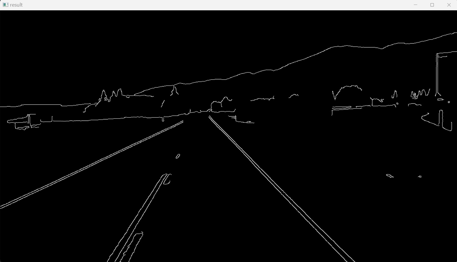
The Python code for implementing the above described five steps of the Canny edge detector is as follows:
import cv2
import numpy as np

image1 = cv2.imread('test_image.jpg')
lane_image = np.copy(image1)
gray_image = cv2.cvtColor(lane_image, cv2.COLOR_BGR2GRAY)
blur_image = cv2.GaussianBlur(gray_image,(5,5),0)
canny_image = cv2.Canny(blur_image, 50, 150)
cv2.imshow("result", canny_image)
cv2.waitKey(0)
After importing the required Python packages, the image is loaded and preprocessed. Then, the Canny edge detector is applied, the cv2.Canny() function, to the single channel, grayscale image to ensure that there is less noise during the process. The first parameter for the cv2.Canny() function is the grayscale blurred image. The second and third parameters are the lower and higher thresholds respectively. Finally, the resulting image with detected edges, Figure 7, is displayed on the screen. It clearly traces the outline of the edges that correspond to the pixels with most sharp changes in intensity. Gradients that exceed the high threshold are traced as bright pixels. Small changes in brightness are not traced at all and accordingly, they are black as they fall below the lower threshold.
3. Region of Interest
A region of interest (often abbreviated ROI) is a sample within a data set identified for a particular purpose. In computer vision, the ROI defines the borders of an object under consideration.
In the previous section’s final image, Figure 7, it could be noticed that after applying the Canny edge detector, there are identified edges in the image that don’t belong to the lane lines. To isolate only the region where lane lines should be identified, a completely-black mask is created, with the same dimensions as the original image, and part of its area is filled with a polygon.
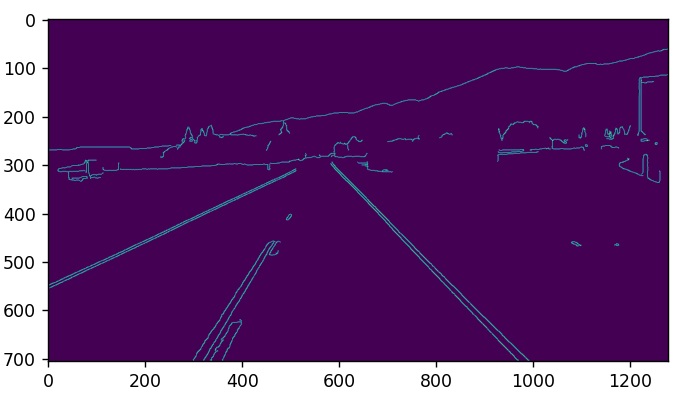
In this project the region of interest is the lane where the vehicle is moving. This region could be specified as a triangle. To accomplish this, first a new function is defined, named canny(), and the previous code is wrapped within it. This function takes as input an image and applies the Canny algorithm to this image and returns the result image as output.
To clarify how the region of interest, the dimensions of the triangle, is isolated, the pyplot subpackage of the Matplotlib package is used, instead of OpenCV, which shows the axes of the figure, as shown in Figure 8.
import cv2
import numpy as np
import matplotlib.pyplot as plt

def canny(image):
    gray_image = cv2.cvtColor(image, cv2.COLOR_BGR2GRAY)
    blur_image = cv2.GaussianBlur(gray_image,(5,5),0)
    canny_image = cv2.Canny(blur_image, 50, 150)
    return canny_image


image1 = cv2.imread('test_image.jpg')
lane_image = np.copy(image1)
canny_image = canny(lane_image)

plt.imshow(canny_image)
plt.show()
Then the region of interest, where the lane lines are to be identified, is traced as a triangle with the following three vertices $(x,y)$: $(200px,700px)$, $(1100px,700px)$ and $(550px,250px)$.
Now the previous code is reversed back to show the image with OpenCV and a new function is defined, region_of_interest(), which takes an image as input and returns the enclosed region of interest, the triangular shape. The region of interest is declared as a 1D NumPy array of vertices.
The height of the image is obtained from the shape() function of the image (2D array of pixels), which is a tuple of two integers $(m, n)$; where $m$ is the number of rows, equals to the height of the image, and $n$ is the number of columns.
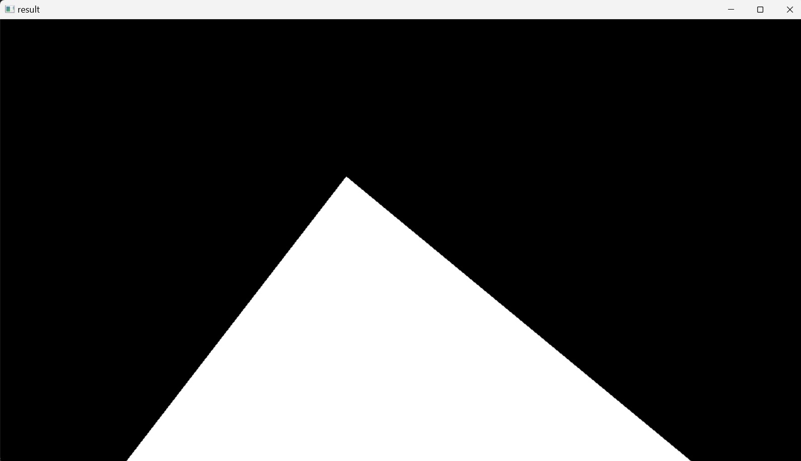
This polygon is applied on a black mask with the same dimensions of the original image. To accomplish this, NumPy’s zero_like() funtion is used, which returns an array of zeros with the same shape and type as the array corresponding to the input image. This mask will have the same number of rows and columns, the same number of pixels, and thus the same dimensions of the original image. However, its pixels will be black as they have zero intensity. Then this mask is filled with the triangle by using OpenCV’s fillPoly() function, which fills an area bounded by one or more polygons, i.e. its second parameter is an array of polygons (here: an array of one polygon). The third parameter in this function specifies the filling color of the polygon, which here is considered to be white. In this way, the area bounded by the defined polygonal contour will be filled with white color. Finally, the modified mask is returned as the output of this function and Figure 9 is displayed on the screen.
This result was achieved by the following Python code:
import cv2
import numpy as np

def canny(image):
    gray_image = cv2.cvtColor(image, cv2.COLOR_BGR2GRAY)
    blur_image = cv2.GaussianBlur(gray_image,(5,5),0)
    canny_image = cv2.Canny(blur_image, 50, 150)
    return canny_image

def region_of_interest(image):
    height = image.shape[0]
    polygons = np.array([
        [[200,height],[1100,height],[550,250]]
        ])
    mask = np.zeros_like(image)
    cv2.fillPoly(mask, polygons, 255)
    return mask

image1 = cv2.imread('test_image.jpg')
lane_image = np.copy(image1)
canny_image = canny(lane_image)

cv2.imshow("result", region_of_interest(canny_image))
cv2.waitKey(0)
The mask image is going to be used now to mask the canny_image image, the result of the Canny edge detector, to show only a specific region of this image, traced by the triangle polygon, and masking the other sections.
This is accomplished by applying the bitwise AND operator (&) between the result image of the Canny operator and the mask image. This operator compares pare of binary numbers and results in zero unless both numbers are ones, as shown in the following table:
| A | B | A & B |
|---|---|---|
| 0 | 0 | 0 |
| 0 | 1 | 0 |
| 1 | 0 | 0 |
| 1 | 1 | 1 |
The bitwise AND operator is applied elementwise between the two images; two arrays of pixels, that have the same dimensions, thus the same number of pixels. The elementwise application of bitwise AND operator operates on each homologous pixel in both arrays, ultimately masking the result image of the Canny edge detector to only show the region of interest traced by the polygon in the mask image.
The mask image is first printed out in its pixel representation, where the triangle polygon is translated to pixel intensities of $255$ and the surrounding regions translate to pixel intensities of $0$. The binary representation of the value $0$ is $0$ and the binary representation of the value $255$ is $11111111$ (the maximum representation value of $8$-bit byte; $2^7+2^6+2^5+2^4+2^3+2^2+2^1+2^0 = 255$). This means that as the surrounding region to the region of interest is black then the binary representation of each pixel intensity in that region would be zero, as the result of bitwise AND operator of all zeros binary number with any other binary number will yield all zeros. This means all pixels in that region will have zero intensity value, black, masking the entire region outside the region of interest. As for the white polygon, the binary representation of each pixel intensity in that region would be one. This means the values of pixel intensities in this region will remain unaffected, as applying bitwise AND operator between all ones binary number and any other binary number will have no effect.
This could be implemented by adding the OpenCV’s bitwise_and() function to the region_of_interest() function in the previous code, which will return the masked_image as its result.
import cv2
import numpy as np

def canny(image):
    gray_image = cv2.cvtColor(image, cv2.COLOR_BGR2GRAY)
    blur_image = cv2.GaussianBlur(gray_image,(5,5),0)
    canny_image = cv2.Canny(blur_image, 50, 150)
    return canny_image

def region_of_interest(image):
    height = image.shape[0]
    polygons = np.array([
        [[200,height],[1100,height],[550,250]]
        ])
    mask = np.zeros_like(image)
    cv2.fillPoly(mask, polygons, 255)
    masked_image = cv2.bitwise_and(image,mask)
    return masked_image

image1 = cv2.imread('test_image.jpg')
lane_image = np.copy(image1)
canny_image = canny(lane_image)
cropped_image = region_of_interest(canny_image)

cv2.imshow("result", cropped_image)
cv2.waitKey(0)
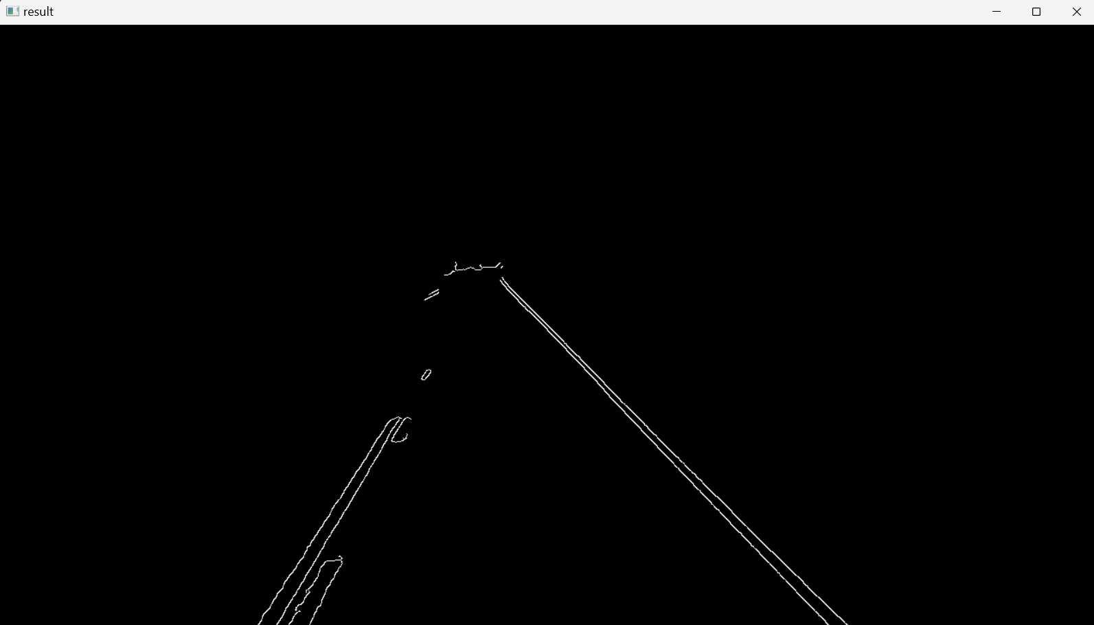
This displays Figure 10 representing the isolated region of interest, due to masking, within the resultant image of the Canny edge detector.
The final step of lane lines detection will be to apply the Hough transform algorithm to detect straight lines in the region of interest and thus identify the lane lines.
4. Hough Transform
In computer vision and image processing an edge detector can be used as a preprocessing stage to obtain image pixels that are on the desired curve, such as straight lines, circles or ellipses, in the image space. Due to imperfections in either the image data or the edge detector, however, there may be missing points or pixels on the desired curves as well as spatial deviations between the ideal line/circle/ellipse and the noisy edge points as they are obtained from the edge detector.
For example, given points that belong to a line, what is the line? How many lines are there? Which points belong to which lines?
To address these questions, Hough transform is used to group the extracted edge points to an appropriate set of lines, circles or ellipses by performing an explicit voting procedure over a set of parameterized image objects.
The simplest case of Hough transform is detecting straight lines. The Main idea is:
- Recording votes for each possible line on which each edge point lies.
- Looking for lines that get many votes.
In a two-dimensional space a straight line is represented on the coordinate plane by the equation:
\[y = mx + b\]This line has two parameters; $m$ and $b$, where $b$ is the $y$-intercept of the line and $m$ is the slope. This line can also be represented in a parameter space, where horizontal axis represents the slopes and the vertical axis represents the $y$-intercepts, as a point $(b, m)$. This parameter space is also known as Hough space.
Considering a single point, $A(x_0,y_0)$, in the two-dimensional space, there are many possible lines that can cross this point, each having different values for $b$ and $m$. In the parameter space, these $b$ and $m$ pairs will represent points that are located on a straight line (collinear points). Thus, a point $A(x_0,y_0)$ in the image spaceis mapped to a line in the parameter space (Hough space):
\[b = -x_0m + y_0\]However, considering two points, $A(x_0,y_0)$ and $B(x_1,y_1)$, in the two-dimensional space, there are many possible lines that can cross each point, each having different values for $b$ and $m$. But, there is one line that crosses both points. This line is represented in the parameter space by a single point $(b, m)$. In other words, this point in the parameter space represents the $(b, m)$ values of a line in two-dimensional space that crosses both points $A(x_0,y_0)$ and $B(x_1,y_1)$. It is the intersection of two lines in the Hough space:
\(b = –x_0m + y_0\) \(b = –x_1m + y_1\)
The same is valid for more than two points in the two-dimensional space.
Considering Figure 7, the result image of applying Canny edge detector, and by taking some points, for example $A$, $B$, $C$, and $D$ in that image space, two-dimensional space, there would be many lines that can cross each of these points. In the parameter space, the Hough space, the lines that crosses $A$, for example, will be represented by points, each with its specific $b$ and $m$ values; $y$-intercept and slope values, and these points will be located on a straight line (collinear points) in the parameter space. The same applies for the points $B$, $C$, and $D$. In this way, there are four lines in the parameter space representing all the lines in the two-dimensional space crossing the four points, $A$, $B$, $C$, and $D$. The intersection of the lines in the parameter space, a point $(b, m)$, will represent a line with parameters $(b, m)$ that crosses all the four points $A$, $B$, $C$, and $D$ in the two-dimensional space, the image space. This idea of identifying possible lines from a series of points is how lines are identified in the image.
However, vertical lines pose a problem. They would give rise to unbounded values of the slope parameter $m$. Thus, for computational reasons, instead of expressing the line $y = mx + b$ with Cartesian coordinate system parameters, $m$ and $b$, it will be expressed in the polar coordinate system with parameters $r$ and $\theta$, and the line equation:
where $r$ is the distance from the origin to the closest point on the straight line, i.e. the perpendicular distance, and $\theta$ is the angle between the $x$ axis and the line connecting the origin with that closest point, increasing in clockwise orientation.
For example, for a vertical line in the two-dimensional space, $\theta = 0$ ⇒ $r=x\cos 0 +y\sin 0 = x$. For a horizontal line in the two-dimensional space, $\theta = 90°$ ⇒ $r=x\cos \frac{\pi}{2} +y\sin \frac{\pi}{2} = y$.
With polar coordinate system representation of a line, for each point $(x,y)$ in the image space, multiple lines can cross this point, each can be represented in the polar coordinate system (here: Hough space) with a point $(\theta,r)$. The set of all straight lines going through the point $(x,y)$ corresponds to a sinusoidal curve in the $(\theta,r)$ plane, which is unique to that point. A set of two or more points that form a straight line will produce sinusoids crossing at the $(\theta,r)$ for that line. Thus, the problem of detecting collinear points in the Hough space can be converted to the problem of finding concurrent curves in the Hough space.
Just like before, if the curves of different points in the image space intersect in Hough space, then these points belong to the same line in the two-dimensional space, and are characterized by a specific $(\theta,r)$. The more curves intersecting in the Hough space means that the line represented by that intersection crosses more points in the image space.
This means that in general, a line can be detected by finding the number of intersections between curves in the Hough space (in the $\theta$ - $r$ plane). The more curves intersecting means that the line represented by that intersection has more points. In general, we can define a threshold of the minimum number of intersections needed to detect a line.
Due to imperfections in either the image data or the edge detector, however, there may be missing points or pixels on the desired lines in the image space, as well as spatial deviations between the ideal line and the noisy edge points as they are obtained from the edge detector. This will cause the curves in the polar space to intersect in more than one point near each other. The purpose of the Hough transform is to address this problem by making it possible to perform groupings of edge points into line candidates by performing an explicit voting procedure. Considering several edge points in the image space, what is the line of best fit for these points? These points have curves in the polar space where each curve represents the lines crossing a single point of those points.
To find the line of best fit for these points, the Hough space (here: the polar space) is split into a grid, each bin inside this grid corresponds to an angle $\theta$ and distance $r$ of a candidate line. Because of the imperfections, several points of intersection could be inside a single bin (single bin represents a line in the image space). Then, for each point of intersection inside the bin a voting procedure is performed inside the bin that it belongs to. Each edge point in image space votes for a set of possible parameters in Hough space. The votes are accumulated in discrete set of bins. The bin with the most votes (the bin with the most number of intersections inside it) is going to be the line in image space crossing these points. The purpose of this technique is to find imperfect instances of points in the image space and the line to which they belong as the vote procedure votes for the line of best fit (the line that has $\theta$ and $r$ values of the bin).
The basic Hough transform algorithm, considering, for example, an image with a line in it, will take the first point of the line. The $(x,y)$ values of this line in the image space are known. In the line equation, the values of $\theta = 0,1,2,….,180$ are put and the value of $r$ is calculated. For every $(\theta,r)$ pair, the value of the vote is incremented by one in its corresponding $(\theta,r)$ bins.
Then the algorithm takes the second point on the line. Does the same as above. Incrementing the the values in the bins corresponding to the resultant $(\theta,r)$. This time, the bin that was previously voted is voted for a second time, so its value is incremented. Which is actually voting the $(\theta,r)$ values. This process continues for every point on the line. At each point, this same bin will be incremented or voted up, while other bins may or may not be voted up. This way, at the end, this bin will have maximum votes, indicating that there is a line in this image at distance $r$ from origin and at angle $\theta$.
In OpenCV, Hough Line transform could be implemented by two kinds: A Standard Hough Line Transform and a Probabilistic Hough Line Transform. The Standard Hough Line Transform is implemented with the function HoughLines(), it is the operation explained thus far. It gives as result a vector of couples $(\theta,r)$. The Probabilistic Hough Line Transform, however, is a more efficient implementation of the Hough Line Transform. It gives as output the extremes of the detected lines $(x_{start}, y_{start}, x_{end}, y_{end})$. In OpenCV it is implemented with the function HoughLinesP().
To continue from the previous code, after detecting the edges of the image by using a Canny detector, the Probabilistic Hough Line Transform is applied, which has the syntax:
linesP = cv2.HoughLinesP(image, 2, np.pi / 180, 100, np.array([]), minLineLength=40, maxLineGap=5)
with the following arguments:
image: The image where the lines are to be detected, thecropped_image.linesP: A vector that will store the parameters $(x_{start}, y_{start}, x_{end}, y_{end})$ of the detected lines.
The next two arguments specify the resolution of the Hough accumulator array, which was described earlier as a grid, an array of rows and columns, which contains the bins that are used to accumulate the votes. Each bin represents a distinct value of $\theta$ and $r$. The next two arguments specify the size of the bins. The larger the bins the less precise the detected lines are going to be and vice versa. However, too small bins can result in inaccuracies and takes longer time to run.
r: The resolution of the parameter $r$ in pixels. Here used $2$ pixels.theta: The resolution of the parameter $\theta$ in radians. Here used $1$ degree precision in radians, i.e.(np.pi/180)threshold: The minimum number of votes (intersections) in a bin to “detect” a line, i.e. to accept a candidate line. Here chosen to be $100$, meaning that the minimum number of intersection in Hough space for a bin needs to be $100$ for it to be accepted as a relevant line in describing the data (the edge points).- An empty placeholder array.
minLineLength: The minimum number of points (pixels) that can form a line. Lines with less than this number of points are disregarded.maxLineGap: The maximum gap between two points (pixels) to be considered in the same line, and thus to be connected instead of being disconnected (broken).
After setting the Hough Line Transform algorithm, the next step is to display the detected lines in the original image by drawing them. For this, a new function is defined, display_lines(), which takes two inputs: An image; in this case the lane_image, onto which it will display the lines, as well as the lines themselves; linesP.
Inside the function display_lines(), the NumPy’s zero_like() funtion is used, which returns an array of zeros with the same shape (dimensions) and type as the array corresponding to the input image. Then, all of the lines that were previously detected by Hough Line Transform will be displayed onto this black image. To accomplish this, first it is checked that the array is not empty; that the lines is not None, then it iterates through the lines, which is a three-dimensional array consisting of the lines and respective two-dimensional rows, $1\times4$, vectors; the $(x_{start}, y_{start}, x_{end}, y_{end})$ parameters of each line. Then each two-dimensional array, parameters of each line, is reshaped to one-dimensional array with four elements followed by assigning these elements to four different variables $x_{1}, y_{1}, x_{2},$ and $y_{2}$ respectively. Finally, each line that the for loop has iterated through is drawn onto the black image line_image by using OpenCV’s line(image, start_point, end_point, line_color, line_thickness) function.
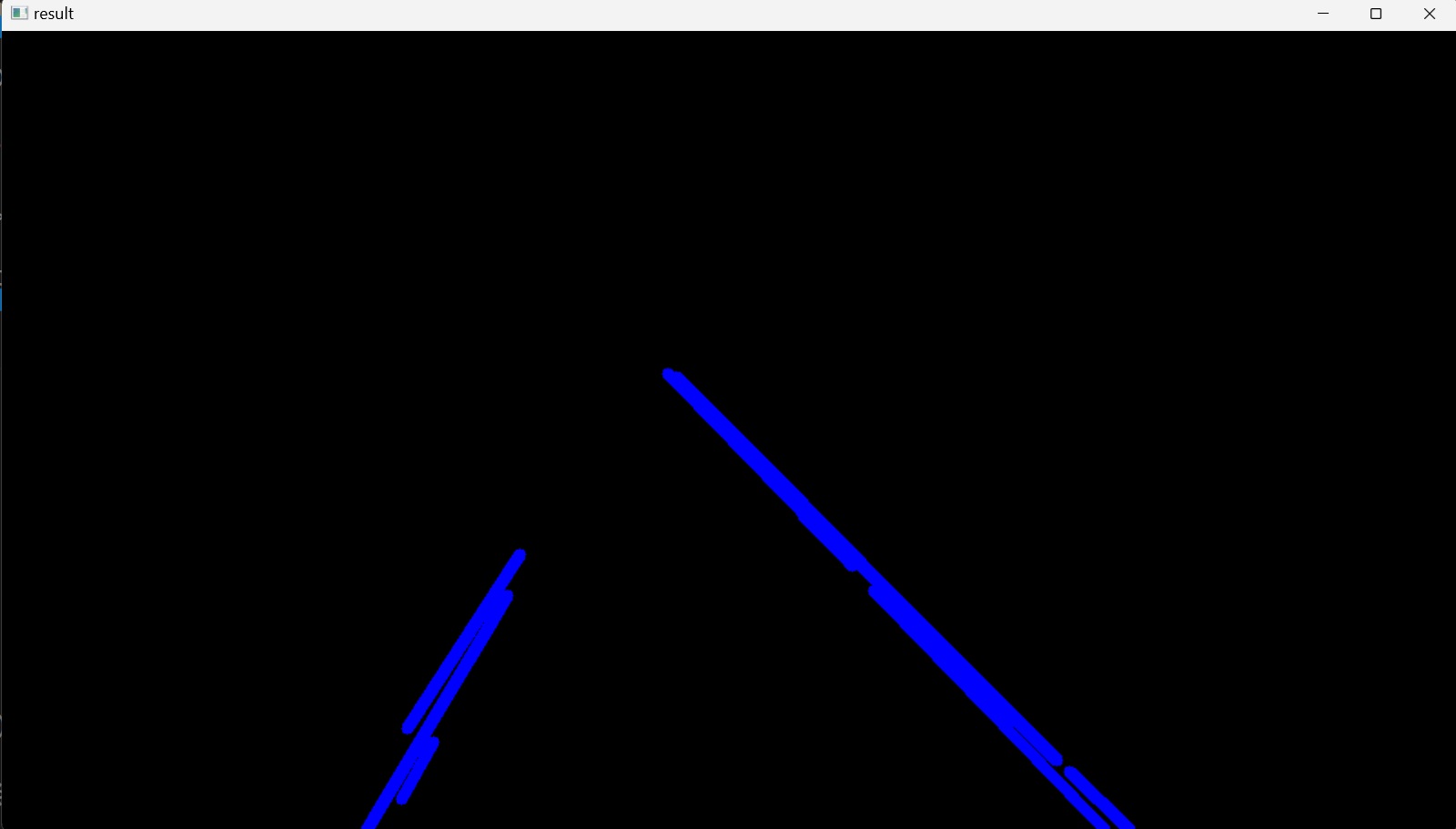
In this way, all the lines that were detected by using the Canny edge detector are drawn onto a black image, Figure 11.
The Python code for this section is as follows:
import cv2
import numpy as np

def canny(image):
    gray_image = cv2.cvtColor(image, cv2.COLOR_BGR2GRAY)
    blur_image = cv2.GaussianBlur(gray_image,(5,5),0)
    canny_image = cv2.Canny(blur_image, 50, 150)
    return canny_image

def display_lines(image, lines):
    line_image = np.zeros_like(image)
    if lines is not None:
        for line in lines:
            x1, y1, x2, y2 = line.reshape(4)
            cv2.line(line_image,(x1,y1),(x2,y2),(255,0,0),10)
    return line_image

def region_of_interest(image):
    height = image.shape[0]
    polygons = np.array([
        [[200,height],[1100,height],[550,250]]
        ])
    mask = np.zeros_like(image)
    cv2.fillPoly(mask, polygons, 255)
    masked_image = cv2.bitwise_and(image,mask)
    return masked_image

image1 = cv2.imread('test_image.jpg')
lane_image = np.copy(image1)
canny_image = canny(lane_image)
cropped_image = region_of_interest(canny_image)
linesP = cv2.HoughLinesP(cropped_image, 2, np.pi / 180, 100, np.array([]), minLineLength=40, maxLineGap=5)
line_image = display_lines(lane_image,linesP)
cv2.imshow("result", line_image)
cv2.waitKey(0)
Finally, the image of the detected lines, displayed on a black image (Figure 11), is blended into the original color image (Figure 1), to show the lines on the lanes. This is done by creating a variable blended_image and assigning to it the output array of the OpenCV’s addWeighted(src1, alpha, src2, beta, gamma[, dst[, dtype]]) function, that has the same size and number of channels as the input arrays; the original color image, lane_image, and the line_image, and blending them by taking the weighted sum between the arrays of these two images. A weight of $0.8$ is assigned to the lane_image to reduce its pixel-intensities to make them a bit darker, and a weight of $1$ is assigned to the line_image according to the following matrix expression:
Where $dst$ is the output array and $gamma$ is a scalar added to each sum. Accordingly, by blending these two images, the line_image will have $20\%$ more weight, more clearly defined, in the blended_image.
In this way, all the lines that were detected by using the Canny edge detector are drawn onto a black image and then blended it into the original color image such that the detected lines are displayed on top of the respective lane lines in the original image, Figure 12. The Python code for this section is as follows:
import cv2
import numpy as np

def canny(image):
    gray_image = cv2.cvtColor(image, cv2.COLOR_BGR2GRAY)
    blur_image = cv2.GaussianBlur(gray_image,(5,5),0)
    canny_image = cv2.Canny(blur_image, 50, 150)
    return canny_image

def display_lines(image, lines):
    line_image = np.zeros_like(image)
    if lines is not None:
        for line in lines:
            x1, y1, x2, y2 = line.reshape(4)
            cv2.line(line_image,(x1,y1),(x2,y2),(255,0,0),10)
    return line_image

def region_of_interest(image):
    height = image.shape[0]
    polygons = np.array([
        [[200,height],[1100,height],[550,250]]
        ])
    mask = np.zeros_like(image)
    cv2.fillPoly(mask, polygons, 255)
    masked_image = cv2.bitwise_and(image,mask)
    return masked_image

image1 = cv2.imread('test_image.jpg')
lane_image = np.copy(image1)
canny_image = canny(lane_image)
cropped_image = region_of_interest(canny_image)
linesP = cv2.HoughLinesP(cropped_image, 2, np.pi / 180, 100, np.array([]), minLineLength=40, maxLineGap=5)
line_image = display_lines(lane_image,linesP)
blended_image = cv2.addWeighted(lane_image, 0.8,line_image,1, 1)
cv2.imshow("result", blended_image)
cv2.waitKey(0)

5. Optimization
The multiple lines displayed on each lane in the original image could be further optimized by averaging the slope and $y$-intercept of these multiple lines into a single line that traces both of the lane lines.
To do this, a new function is defined; average_slope_intercept(), which takes two images as input. The original colored lane_image and the detected lines linesP are passed to this function by defining a new variable averaged_lines, which equals to the return value of this function. Inside the function definition, two empty lists are declared, left_fit and right_fit, to contain the coordinates of the averaged lines displayed on the left and right side of the lane in the region of interest respectively. This is done by iterating through every line and reshaping each line into one-dimensional array with four elements and assigning the variables $x_{1}, y_{1}, x_{2},$ and $y_{2}$ to the elements respectively. These are the start and end points of a line in the two-dimensional image space, but what is required are the slope and the $y$-intercept of this line. To find these values, a new variable, parameters, is set to equal to the return values of NumPy’s np.polyfit() function, which fits a first degree polynomial (a line) to the points $(x_{1}, y_{1})$ and $(x_{2}, y_{2})$ and returns a vector of coefficients describing the slope and the $y$-intercept of the line, the first and second elements of the vector respectively.
The function np.polyfit() needs three parameters: the $y$ and $x$ values of previously defined start and end points, and an integer, here: $1$, which defines the degree of the polynomial to fit the points. Accordingly, the parameters of the linear function are obtained and assigned to the variables slope and y_intercept respectively. Then, after each iteration, each line is checked whether it corresponds to a line on the left side of the lane or the right. It is important to note here that in OpenCV coordinate system, the $Y$-axis is oriented downward, also, from the definition of a slope, a line has a positive slope when its $y$ values increase as its $x$ values increase. It could be noticed from the images that all the lines in the region of interest are in the same direction, either slanted a bit to the left, on the right side of the lane (positive slope value), or slanted a bit to the right, on the left side of the lane (negative slope value). Based on this, lines with positive slopes are appended to the right_fit list and lines with negative slopes are appended to the left_fit list.
Python’s appended method takes a single argument as input, an item, and adds this item to the end of the list. In this case, items added to the lists are tuples (slope, y_intercept), so both lists have the shape of a matrix with several rows and two columns. Then, as the $for$ loop iteration ends, the values in each list are averaged into a single slope and $y$-intercept by the NumPy’s average() function, which returns the average along the specified axis. In this case, it takes as input a list and returns the average of this list along the first axis running vertically downwards across the rows (axis $0$). The result of this is two arrays, each representing the average slope and $y$-intercept of a single line to the left side and right side of the lane respectively.
After getting the slopes and $y$-intercepts of the left and right lines, the next step is to specify the coordinates where the lines should be placed; the $x_{1}, y_{1}, x_{2},$ and $y_{2}$ for each line. To do this, a new function is defined; make_coordinates(), which has the arguments image and line_parameters as input. line_parameters are the slope and the $y$-intercept of both the left and right lines, in this case, the left_fit_average and the right_fit_average, each a list of two elements; a slope value and a $y$-intercept value. Then the start and end points of the lines are specified by setting the y1 = image.shape[0], where the shape() method returns a tuple value that indicates the lengths of the corresponding array dimensions; i.e. the number of corresponding elements. In this case, y1 = image.shape[0] sets the number of image pixels only along the vertical $Y$ axis, which is directed downwards, equal to y1. $y_2$ is set to equal $\frac{3}{5}$ times the length of $y_1$. This means that both lines will start from the bottom of the image and go three-fifths of the distance upwards. $x_1$ and $x_2$ are determined algebraically from the equation of the respective line.
After obtaining all the coordinates, the make_coordinates() function’s result is returned back to the two callers, left_line and right_line within the average_slope_intercept() function, as NumPy arrays. Then the average_slope_intercept() function’s result, the two averaged lines, is returned as NumPy array to the caller, the variable averaged_lines.
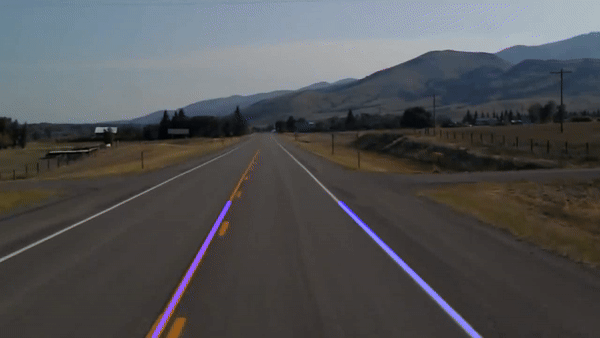
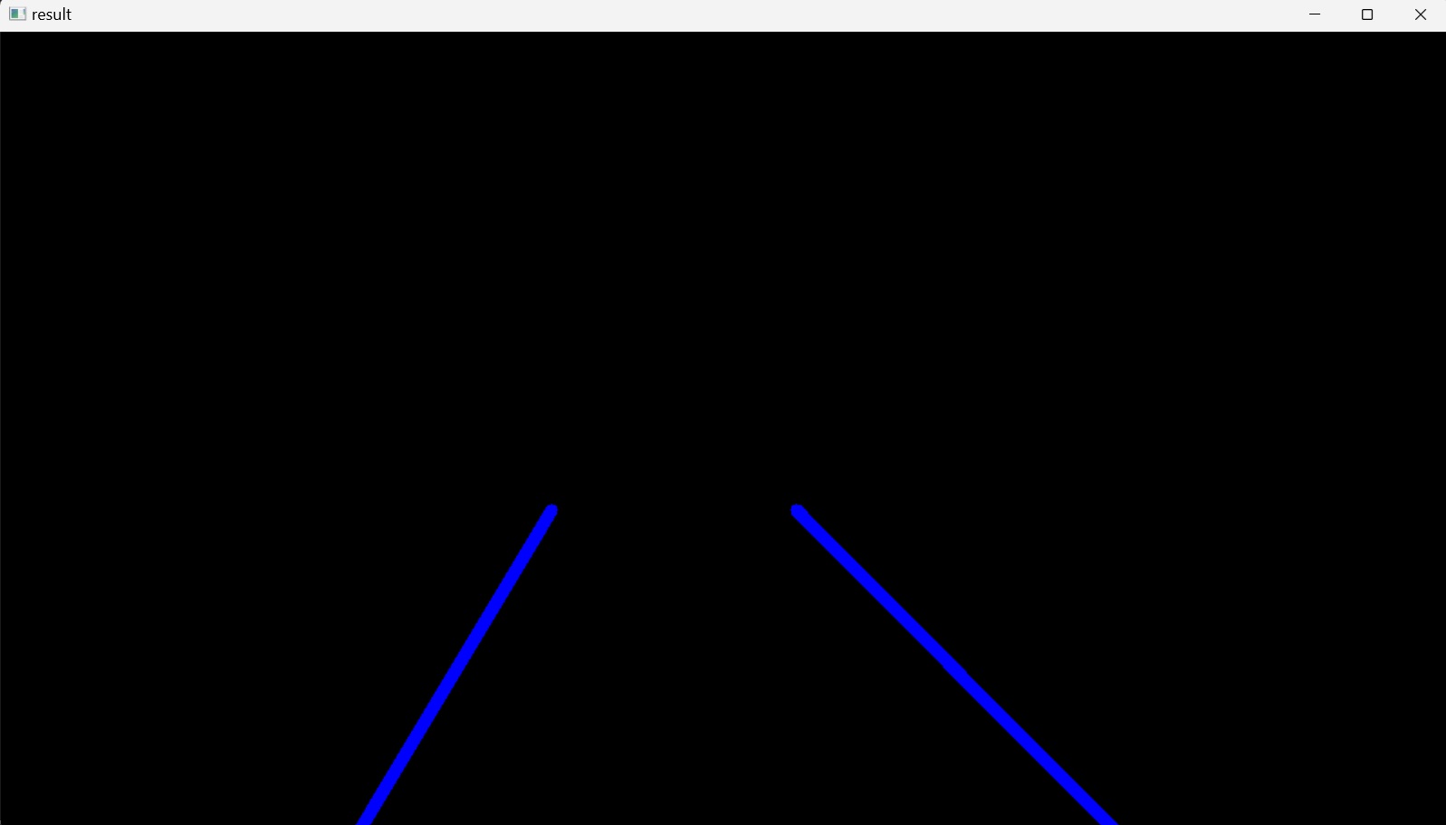
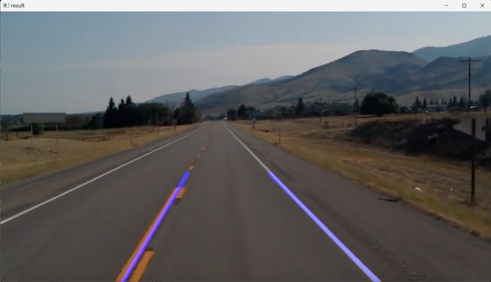
Finally, the averaged_lines is passed to the variable line_image instead of previously passed linesP, and the result line_image is displayed on the screen by the line of code cv2.imshow("result", line_image), Figure 13.
To show the blended image of the averaged lines into the original image, Figure 13, the line of code cv2.imshow("result", line_image) is changed to cv2.imshow("result", blended_image).
Here the code could be improved by changing the previously defined display_lines() function’s code:
def display_lines(image, lines):
    line_image = np.zeros_like(image)
    if lines is not None:
        for line in lines:
            x1, y1, x2, y2 = line.reshape(4)
            cv2.line(line_image,(x1,y1),(x2,y2),(255,0,0),10)
    return line_image
by removing the line of code x1, y1, x2, y2 = line.reshape(4) in the forloop and replacing the value line, which accesses each value of lines on each iteration, with x1, y1, x2, y2. This is possible now because the reshaping or flattening of each line is already carried out in the average_slope_intercept() function. Thus, there is no need to reshape or flatten each line in the display_lines() function again. So, the code of the display_lines() is changed to:
def display_lines(image, lines):
    line_image = np.zeros_like(image)
    if lines is not None:
        for x1, y1, x2, y2 in lines:
            cv2.line(line_image,(x1,y1),(x2,y2),(255,0,0),10)
    return line_image
The final code for this section is as follows:
import cv2
import numpy as np

def make_coordinates(image, line_parameters):
    slope, y_intercept = line_parameters
    y1 = image.shape[0]
    y2 = int(y1*(3/5))
    x1 = int((y1 - y_intercept)/slope)
    x2 = int((y2 - y_intercept)/slope)
    return np.array([x1, y1, x2, y2])

def average_slope_intercept(image, lines):
    left_fit = []
    right_fit = []
    for line in lines:
        x1, y1, x2, y2 = line.reshape(4)
        parameters = np.polyfit((x1, x2), (y1, y2), 1)
        slope = parameters[0]
        y_intercept = parameters[1]
        if slope < 0:
            left_fit.append((slope, y_intercept))
        else:
            right_fit.append((slope, y_intercept))
    left_fit_average = np.average(left_fit, axis=0)
    right_fit_average = np.average(right_fit, axis=0)
    left_line = make_coordinates(image, left_fit_average)
    right_line = make_coordinates(image, right_fit_average)
    return np.array([left_line, right_line])


def canny(image):
    gray_image = cv2.cvtColor(image, cv2.COLOR_BGR2GRAY)
    blur_image = cv2.GaussianBlur(gray_image,(5,5),0)
    canny_image = cv2.Canny(blur_image, 50, 150)
    return canny_image

def display_lines(image, lines):
    line_image = np.zeros_like(image)
    if lines is not None:
        for x1, y1, x2, y2 in lines:
            cv2.line(line_image,(x1,y1),(x2,y2),(255,0,0),10)
    return line_image

def region_of_interest(image):
    height = image.shape[0]
    polygons = np.array([
        [[200,height],[1100,height],[550,250]]
        ])
    mask = np.zeros_like(image)
    cv2.fillPoly(mask, polygons, 255)
    masked_image = cv2.bitwise_and(image,mask)
    return masked_image

image1 = cv2.imread('test_image.jpg')
lane_image = np.copy(image1)
canny_image = canny(lane_image)
cropped_image = region_of_interest(canny_image)
linesP = cv2.HoughLinesP(cropped_image, 2, np.pi / 180, 100, np.array([]), minLineLength=40, maxLineGap=5)
averaged_lines = average_slope_intercept(lane_image, linesP)
line_image = display_lines(lane_image, averaged_lines)
blended_image = cv2.addWeighted(lane_image, 0.8,line_image,1, 1)
cv2.imshow("result", blended_image)
cv2.waitKey(0)
6. Identifying Lane Lines in a Video
In the previous sections, the lane lines detection algorithm was designed and implemented successfully in identifying lane lines in an image. In this section, the same algorithm will be used to identify lane lines in a video.
To capture the video into the workspace, the OpenCV’s VideoCapture() function is used whose argument is either the camera’s index (starting from $0$ for the first camera) or the name of a video file. Here a previously captured video file is used. This function returns a VideoCapture object cap.
A video is a collection of images; ‘frames’. Thus, to process a video stream, the program loops through all the frames in the video sequence and then processes them one at a time.
For this, an infinite while loop is set up, which, after initializing the VideoCapture object; cap.isOpen(), reads (grabs and decodes) every successive video frame from the cap object with the help of read() method and returns a tuple, where the first element is a Boolean and the next element is the actual video frame. When the first element, success is True, indicating that the read was successful, the second element, the current frame in the video, is returned and assigned to the a variable named frame1. Then, after checking that the condition of the next if statement is False, the frame1 is assigned to a new variable named frame, and the value of this variable is passed through the algorithm for edge detection. The reason for taking this extra step, and not directly passing the frame1 into the algorithm, is that at the end of the video, the read() method inside the while loop passes an empty video frame to the algorithm, as there are no more frames, and this causes an error message in the terminal window: _src.empty() in function 'cv::cvtColor'. To avoid this, the if statement for checking the Boolean value is added so that when the success is False, for example, at the end of the video, the loop breaks and the frame1 doesn’t pass to the algorithm.
In the next steps, the desired operations on the video frame frame are performed, like described in the previous sections, and finally, each frame is displayed by the cv2.imshow() function, Figure 15. For this, the previously coded algorithm is cut and pasted in the VideoCapture loop and the previous static image input to the functions canny(), average_slope_intercept() and display_lines() are changed with the video frame frame, as shown in the final code below.
The waitKey() function’s parameter is also changed from $0$ to $1$ millisecond, for the program to wait $1$ between each frame. Because if it is $0$, then the program will wait infinitely between each frame in the video (will be frozen). Also, to let the output video, i.e. the while loop, to close upon pressing a key, in this case q, because otherwise it won’t close until it is through the complete duration of the video, the waitKey() is added to the code within an if statement.
The waitKey() returns a $32$-bit integer value of the pressed key. This value is compared to the numeric encoding of the keyboard’s q Unicode character, which corresponds to the key to be pressed to break the loop. The integer value of the Unicode character q is obtained from the built-in function ord(). The bitwise AND operation & 0xFF is added to effectively mask the integer value returned by waitKey().
In hexadecimal (base $16$), F is equivalent to $1111$ in the binary numeral system. Python uses the prefix 0x for numeric constants represented in hexadecimal. So, 0xFF is $11111111$ in binary, which represents the decimal value $255$. Thus, 0xFF is an identity element for the bitwise AND operation. So, if the pressed key’s decimal value is larger than $255$, i.e. its binary representation is longer than $8$-bits it takes only the last $8$ bits from the returned value of waitKey() and compares it with the integer value of the Unicode character q. In other words, if this returned value is less than $255$, it won’t be changed. Otherwise, it will be the last $8$ bits of the returned value. This is done to insure cross-platform compatibility when doing the comparison.
After the loop is broken, the video file is closed by calling cap.release() and all windows that were created while running this program are destroyed by calling cv2.destroyAllWindows().
import cv2
import numpy as np

def make_coordinates(image, line_parameters):
    slope, y_intercept = line_parameters
    y1 = image.shape[0]
    y2 = int(y1*(3/5))
    x1 = int((y1 - y_intercept)/slope)
    x2 = int((y2 - y_intercept)/slope)
    return np.array([x1, y1, x2, y2])


global_left_fit_average = []
global_right_fit_average = []
def average_slope_intercept(image, lines):
    left_fit = []
    right_fit = []
    global global_left_fit_average
    global global_right_fit_average

    if lines is not None:
        for line in lines:
            x1, y1, x2, y2 = line.reshape(4)
            parameters = np.polyfit((x1, x2), (y1, y2), 1)
            slope = parameters[0]
            y_intercept = parameters[1]
            if slope < 0:
                left_fit.append((slope, y_intercept))
            else:
                right_fit.append((slope, y_intercept))
    if (len(left_fit) == 0):
        left_fit_average = global_left_fit_average
    else:
        left_fit_average = np.average(left_fit, axis=0)
        global_left_fit_average = left_fit_average

    # left_fit_average = np.average(left_fit, axis=0)
    right_fit_average = np.average(right_fit, axis=0)
    global_right_fit_average = right_fit_average
    left_line = make_coordinates(image, left_fit_average)
    right_line = make_coordinates(image, right_fit_average)
    return np.array([left_line, right_line])


def canny(image):
    gray_image = cv2.cvtColor(image, cv2.COLOR_BGR2GRAY)
    blur_image = cv2.GaussianBlur(gray_image,(5,5),0)
    canny_image = cv2.Canny(blur_image, 50, 150)
    return canny_image


def display_lines(image, lines):
    line_image = np.zeros_like(image)
    if lines is not None:
        for x1, y1, x2, y2 in lines:
            cv2.line(line_image,(x1,y1),(x2,y2),(255,0,0),10)
    return line_image

def region_of_interest(image):
    height = image.shape[0]
    polygons = np.array([
        [[200,height],[1100,height],[550,250]]
        ])
    mask = np.zeros_like(image)
    cv2.fillPoly(mask, polygons, 255)
    masked_image = cv2.bitwise_and(image,mask)
    return masked_image

# image1 = cv2.imread('test_image.jpg')
# lane_image = np.copy(image1)
# canny_image = canny(lane_image)
# cropped_image = region_of_interest(canny_image)
# linesP = cv2.HoughLinesP(cropped_image, 2, np.pi / 180, 100, np.array([]), minLineLength=40, maxLineGap=5)
# averaged_lines = average_slope_intercept(lane_image, linesP)
# line_image = display_lines(lane_image, averaged_lines)
# blended_image = cv2.addWeighted(lane_image, 0.8,line_image,1, 1)
# cv2.imshow("result", blended_image)
# cv2.waitKey(0)

cap = cv2.VideoCapture("test2.mp4")
while(cap.isOpened()):
    success, frame1 = cap.read()
    if success == False:
        break
    frame=frame1
    canny_image = canny(frame)
    cropped_image = region_of_interest(canny_image)
    linesP = cv2.HoughLinesP(cropped_image, 2, np.pi / 180, 100, np.array([]), minLineLength=40, maxLineGap=5)
    averaged_lines = average_slope_intercept(frame, linesP)
    line_image = display_lines(frame, averaged_lines)
    blended_image = cv2.addWeighted(frame, 0.8,line_image,1, 1)
    cv2.imshow("result", blended_image)
    if cv2.waitKey(1) & 0xFF == ord('q'):
        break
cap.release()
cv2.destroyAllWindows()